Systems & Convolution
System Definitions
What is a system?
A systems is "a set of interacting or interdependent components that form an intergrated whole"
There are several other such definitions in the literature in various fields such as mechanics, theromodynamics, etc.
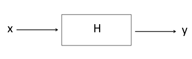
For us a system is a box that takes in a signal $x$ as an input and outputs a signal $y$ as illustrated below:
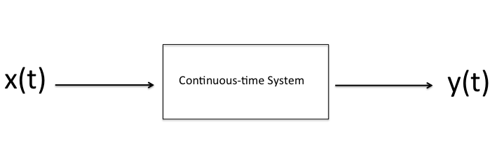
CONTINUOUS-TIME systems process
inputs and
outputs of
continuous-time signals.
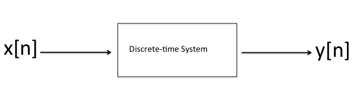
DISCRETE-TIME systems process inputs and outputs of discrete-time signals.
We can repesent the system by an operator $H$:
$y = H\ \cdot x$
The notation indicates that y changes with x. For example the nature of the operator specifies the type of system.
Back
Interconnection of Systems
Systems can be combined to form more complex systems otherwise known as the interconnection of systems.
We will generically use $x$ and $y$ without $x(t)$ and $x[n]$ in this discussion with the understanding that this notation
applies to both CT and DT systems.
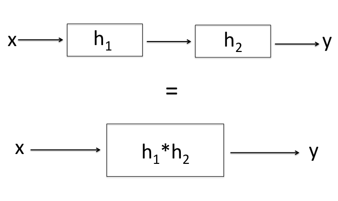
Series/Cascade Interconnection
A series or casade interconnection is the results of an input $x$ into system $H_1$ which results in an output $z$ that
is in turn the input for system $H_2$ which results in an output $y$ as illustrated below.
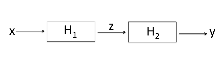
A cascade system can mathematically be represented as:
\[z = H_1 \cdot x\]
\[y = H_2 \cdot z\]
\[ y = H_1 \cdot H_1 \cdot x
\]
One key question to ask yourself is, does the order of systems $H_1$ and $H_2$ matter? It does indeed matter.
As illustrated below the first cascade system is not necessarily equal to the second cascade system.
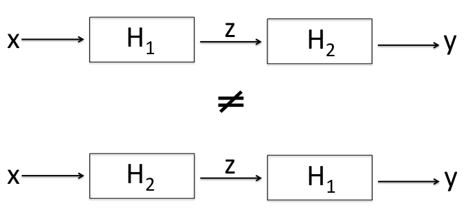
\[\text{Case 1: } y = H_2 \cdot H_1 \cdot x\]
\[\text{Case2: }y = H_1 \cdot H_2 \cdot x\]
In general
\[H_1 \cdot H_2 \neq H_2 \cdot H_1
\]
exept for some special cases
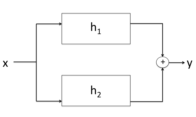
Parallel Interconnection
In a parallel interconnection the input $x$ goes into both systems $H_1$ and $H_2$ simulatenously. The output
from both systems are added together to produce the resulting output $y$ which is illustrated below:
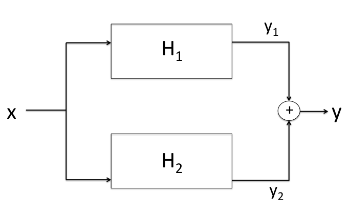
Mathematically:
\[y_1 = H_1 \cdot x \textbf{ and } y_2 = H_2 \cdot x \]
\[y = y_1 + y_2 \]
\[y = H_1 \cdot + H_2 \cdot x\]
\[y = (H_1 + H_2) \cdot x\]
Feedback Interconnection
In a feedback interconnection the output itselfs affects the output.
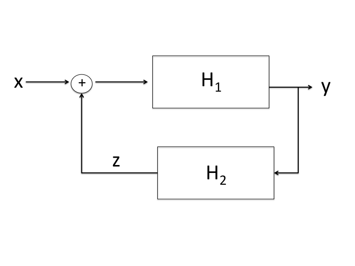
\[y = (x + z) \cdot H_1\]
\[z = H_2 \cdot y\]
\[y = H_1 \cdot (x + H_2 \cdot y)\]
Simple System Examples
Identity Transform
The output is exactly the input. This is a "do-nothing" system
\[y = H \cdot x = x \text{ Notation: } H = I\]
\[x = I \cdot x\]
Delay
The delay system introduces a delay in the signal.
\[y = H \cdot x = x(t - \tau) \text{(CT)}\]
\[y = H \cdot x = x[n - N] \text{(DT)}\]
Back
System Properties
Memoryless System
A system is said to be memoryless if its output at any time depends only on its input at the same instant
with no reference to input values at other times. Mathematically this can be illustrated in CT and DT.
\[x(t_o) \rightarrow y(t_o) \text{ (CT)}\]
\[x[n_o] \rightarrow y[n_o] \text{ (DT)}\]
EXAMPLES
Memoryless
- $y(t) = 4 * x(t)$
- $y[n] = x^2[n]$
Non-memoryless Systems
- $y[n] = \sum_{-\infty}^{n}x[n]$
- $y[n] = x[n-k]$ for $k \neq 0$
Back
Invertibility
A system H is said to be invertible if for every $y = H \cdot x$. There exist another system $\bar{H}$ such that $x$ can be recovered from y
as $x = \bar{H} \cdot y$
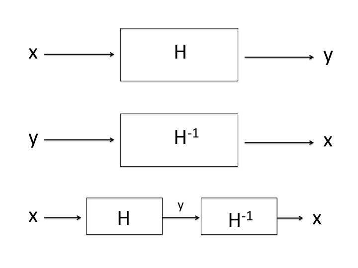
\[x = \bar{H} \cdot H \cdot x\]
where
\[\bar{H} \cdot H = I \text{ (identity)}\]
EXAMPLES
Invertible Systems
- $y(t) = 4x(t)$
- $x(t) = \frac{1}{4}y(t)$ is the inverse
- $y[n] = \sum_{-\infty}^{n} x[n]$
- $x[n] = y[n] - y[n-1]$ is the inverse
Non-invertible Systems
- $y(t) = x^{2}(t)$
- Cannot determine sign of input from knowledge of output so the system in not invertible
- $ y[n] =
\begin{cases}
\sum_{k=0}^{n} x[k], & n \ge 0 \\
0, & n < 0
\end{cases}$
- For $n < 0$ regardless of the value of $n$, $y[n]$ is 0 so this system not invertible
Back
Causality
A system is said to be causal if the output at any time depends only on the input prior to & until that time.
The system does not anticipate the future. Mathematically we say a system is causal if:
CT
\[ \text{For }y_{1}(t) = H \cdot x_{1}(t) \textbf{ and } y_{2}(t) = H \cdot x_{2}(t)\]
\[ \text{If }x_1(t) = x_2(t) \text{ for } t \le t_o\]
\[ \text{then }y_1(t) = y_2(t) \text{ for } t \le t_o\]
DT
\[ \text{For }y_{1}[n] = H \cdot x_{1}[n] \textbf{ and } y_{2}[n] = H \cdot x_{2}[n]\]
\[ \text{If }x_1[n] = x_2[n] \text{ for } n \le n_o\]
\[ \text{then }y_1[n] = y_2[n] \text{ for } n \le n_o\]
EXAMPLES
Two forms of "moving average" systems can make a distinction between causual & non-causual systems.
Causal "moving average"
\[y[n] = \frac{1}{3}\{x[n-2] + x[n-1] + x[n]\}\]
Here the output only relys on prior and current values of the input. It is therefore
causual.
Non-causal Systems
\[y[n] = \frac{1}{3}\{x[n-1] + x[n] + x[n+1]\}\]
Here the ouput relys on "anticipated" values of the input therefore this system is
not causual.
Anti-Causal
Similarly defined to that of causality except the output depends only on current and future samples
\[\text{If }x_1[n] = x_2[n] \text{ for } n \ge n_o \Longrightarrow y_1[n] = y_2[n] \text{ for }n \ge n_o\]
Back
Stability
A system is said to be stable if for every input that is bounded in amplitude the output is also bounded in amplitude.
\[\text{For every } y = H \cdot x\]
CT
\[\text{If } |x(t)| < B \text{ } \forall t \Longrightarrow |y(t)| < V \text{ }\forall t\]
For example if every $x(t)$ is known to be less than some value $B$, then there's some value $V$ such that every $|y(t)| < $V
DT
\[\text{If } |x[n]| < B \text{ } \forall n \Longrightarrow |y[n]| < V \text{ } \forall n\]
EXAMPLES
- $y[n] = \sum_{-\infty}^{n} x[n]$
is not stable because if $x[n] = 1$, $y[n]$ grows without bounds
- $y(t) = e^{x(t)}$
\[ \text{If } |x(t)| < B \text{ or } -B < x{t} < B\]
\[e^{-B} < y(t) < e^{B}\]
is stable because $y(t)$ is bounded
Back
Time Invariance (Shift-Invariance)
A time-invariant system is one in which a shift of the input results in a corresponding shift of the output.
Mathmatically a system is time-invariant if for:
\[x(t) \rightarrow y(t) \Longrightarrow x(t-t_0) \rightarrow y(t-t_0) \text{ (CT)}\]
\[x[n] \rightarrow y[n] \Longrightarrow x[n -n_0] \rightarrow y[n-n_0] \text{(DT)}\]
Time-invariant DT systems are called SHIFT INVARIANT
EXAMPLES
Is $y[n] = a_0x [n] a_1x[n-1] + \ldots + a_kx[n-k]$ is shift invariant?
Proof:
\[\text{Let } x_2[n] = x_1[n-n_o]\]
\[\text{Let } x_1[n] \rightarrow y_1[n] \]
Response to $x_1$
\[y_1[n] = a_0x_1[n] + a_1 x_1[n-1] + \ldots + a_k x_1[n-k]\]
\[y_1[n-n_o] = a_0x_1[n-n_o] + a_1 x_1[n- n_o -1] + \ldots + a_k x_1[n- - n_o -k]\]
Respone to $x_2$
\[y_2[n] = a_0 x_2[n] + a_1 x_2[n-1] + \ldots + a_k x_2[n-k]\]
\[y_2[n]= a_0 x_2[n-n_o] + a_1 x_2[n-n_o-1] + \ldots + a_k x_2[n-n_0-k]\]
So shift invariant because
\[x_1[n-n_o] \rightarrow y_1[n-n_o]\]
Is $y[n] = n \cdot x[n]$ shift invariant
\[\text{Let } x_2[n] = x_1[n-n_0]\]
\[x_1[n] \rightarrow y_1[n] = n \cdot x_1[n]\]
\[y_1[n-n_0] = (n-n_0) x_1[n-n_0]\]
\[x_2[n] \rightarrow y_2[n] = n x_2[n]\]
This system is not shift invariant because
\[ n x_1[n-n_0] \neq y_1[n-n_0]\]
Back
Linearity
A system is said to be linear if it posses the following property two properties:
- Homogeniety:
\[ax_1\rightarrow y_1\]
-
Additivity:
\[x_1 + x_2 \rightarrow y_1 + y_2\]
If a system has both of these properties it is lines
\[ax_1(t) + bx_2(t) \rightarrow ay_1(t) + by_2(t) \text{ (CT)}\]
\[ax_1[n] + bx_2[n] \rightarrow ay_1[n] + by_2[n] \text{ (DT)}\]
EXAMPLES
- Is $y(t) = tx(t)$ linear?
Proof:
\[x_1(t) \rightarrow y_1(t) = tx_1(t)\]
\[x_2(t) \rightarrow y_2(t) = tx_2(t)\]
\[x_3(t) = ax_1(t) +bx_2(t)\]
\[x_3(t) \rightarrow y_3(t) = tx_3(t)\]
\[
\begin{align*}
y_3(t) &= t(ax_1(t)) + bx_2(t) \\
&=atx_1(t) + btx_2(t) \\
&= ay_1(t) + by_2(t)
\end{align*}
\]
So linear because $ax_1(t) +bx_2(t) \rightarrow ay_1(t) + by_2(t)$
-
Is $y(t) = x^2(t)$ linear?
Proof:
\[x_1(t) \rightarrow y_1(t) = x_1^{2}(t)\]
\[x_2(t) \rightarrow y_2(t) = x_2^{2}(t)\]
\[x_3(t) = ax_1(t) +bx_2(t)\]
\[
\begin{align*}
x_3(t) \rightarrow y_3(t) &= x_3^{2}(t) \\
&=(ax_1(t) + bx_2(t))^{2} \\
&=a_2x_1^{2}(t) +b^2x_2^2(t) + 2abx_1(t)x_2(t) \\
&=a^2y_1(t) +b^2y_2(t) + 2abx_1(t)x_2(t)
\end{align*}\]
So the above system is not linear because an added and scaled version of the input does not result
in an added scaled version of the output.
Back
Linear Shift-Invariant (Linear Time-Invariant) Systems
A system is said to be LSI (LTI for CT) if it is both linear annd shift- (time-) invariant.
For such a system:
\[x_1[n] \rightarrow y_1[n]\]
\[x_2[n] \rightarrow y_2[n]\]
\[a x_1[n-n_o] + b x_2 [n-n_o] \rightarrow a y_1[n-n_o] + b y[n-n_o]\]
EXAMPLES
To prove LSI, show that it is both linear & SI
Back
Impulse Response and Convolution
Let us now consider how LTI systems respond to inputs
Recall any signal $x[n]$ can be written as:
\[x[n] = \sum_{k=-\infty}^{\infty}x[k]\delta[n-k]\]
Also recall the definition of an LSI system
CT
\[x_1(t) \rightarrow y_1(t)\]
\[x_2(t) \rightarrow y_2(t)\]
\[a x_1(t-\tau) + b x_2(t-\tau) \rightarrow a y_1(t-\tau) + b y_2(t-\tau)\]
DT
\[x_1[n] \rightarrow y_1[n]\]
\[x_2[n] \rightarrow y_2[n]\]
\[a x_1[n-k] + b x_2[n-k] \rightarrow a y_1[n-k] + b y_2[n-k]\]
Consider an LSI system:
$x[n] \rightarrow y[n]$
Specifically consider how the system responds to an impulse input:
$\delta[n] \rightarrow h[n]$
We call $h[n]$ the impulse response of the system. It is the ouput it generates in response to an input impulse.
We can define an impulse response to CT systems as well. Let us now see how it responds to an arbitrary signal x[n].
\[
\begin{align*}
x[n] &= \sum_{k=-\infty}^{\infty}x[k]\delta[n-k] \\
&= x[0] \delta[n] \rightarrow x[0]h[n] \\
&= x[1] \delta[n-1] \rightarrow x[0]h[n-1] \\
&= x[-1] \delta[n+1] \rightarrow x[0]h[n+1] \\
&= x[2] \delta[n-2] \rightarrow x[0]h[n-2] \\
&= x[-2] \delta[n+2] \rightarrow x[0]h[n+2] \\
&. \\
&. \\
&. \\
&. \\
\end{align*}
\]
\[x[n] = \sum_{k=-\infty}^{\infty}x[k]\delta[n-k] \rightarrow \sum_{k=-\infty}^{\infty}x[k]h[n-k]\]
\[\text{Since } x[n] = \sum_{k=-\infty}^{\infty}x[k]\delta[n-k]\]
\[x[n] \rightarrow y[n] = \sum_{k=-\infty}^{\infty}x[k]h[n-k]\]
\[y[n] = \sum_{k = -\infty}^{\infty}x[k] h[n-k]\]
Implications:
In an LSI system the response of the system to any input is completely determined from its impulse response.
In other words, the system is completely specified by its impulse response h[n].
The equation relating x to y is :
\[y[n] = \sum_{k=-\infty}^{\infty}x[k]h[n-k]\]
is knowns as the CONVOLUTION of $x[n]$ & $h[n]$
It is usually represented a $y[n] = H[n] * x[n]$
A similar relation can be found for CT LTI systems
\[\text{If } \delta(t) \rightarrow h(t)\]
\[x(t) = \int_{-\infty}^{\infty}x(\tau)\delta(t - \tau)d \tau\]
\[y(t) = \int_{-\infty}^{\infty}x(\tau)h(t-\tau)d\tau\]
Understanding the Convolution
So to visualize how to compute $y[n]$ we flip h[n] and shift it forward one step at a time. At each shift $n$ we multiple the $x[k]$ &
$h[n-k]$ sample by sample and add the samples up to get $y[n]$
Click here to visualize convolution. (Courtesy of Amir Asif from York Unviersity)
Back
Properties of Convolution
Commutativity
\[y[n] = h[n] * x[n] = \sum_{k=-\infty}^{\infty}x[k]h[n-k]\]
\[\text{Let } r = n-k \text{ so } k = n-r\]
\[k = \infty \Rightarrow r = -\infty\]
\[k = -\infty \Rightarrow r = \infty\]
\[
\begin{align*}
y[n] &= \sum_{r - \infty}^{\infty}x[n-r]h[r] \\
&= \sum_{r = -\infty}^{\infty}h[r]x[n-r] \\
&= h[n] * x[n]
\end{align*}\]
Convolution is communative where $x*h = h*x$ so does not matter which is the system ad which is the impulse response
Associativity
\[x * h_1 * h_2 = (x * h_1) * h_2 = x * (h_1 * h_2)\]
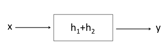
Distributivity
\[
\begin{align*}
y &= x * h_1 + x * h_2 \\
&= \sum_{k}^{}x[k]h_1[n-k] + \sum_{k}^{}x[k]h_2[n-k] \\
&=\sum_{k}^{}x[k](h_1[n-k]+h_2[n-k]) \\
&=x * (h_1 + h_2)
\end{align*}
\]
 \[=\]
\[=\] 
LSI systems are:
- Commutative
- Associative
- Distributive
Back
Infinite Impulse Response (IIR) & Finite Impulse Response (FIR)
In general the impulse response of a system is:
\[y[n] = \sum_{k=0}^{K}a_kx[n-k]\]
is $K+1$ steps for for:
\[y[n] = \sum_{k=-R}^{K}a_kx[n-k]\]
is for R+K-1 steps
If R & K are finite, the impulse response of such a system is finite in length. Such a system is called a FINITE IMPULSE RESPONSE (FIR)system
If $K+R = \infty$, the impulse response is infinitly long and the system is called a INFINITE IMPULSE RESPONSE (IIR) system
Consider the following system
\[y[n] = a_0x[n] + b_1y[n-1] b_2y[n-2]\]
This is a recusive equation and if we expand the above equation we get:
\[y[n-1] = a_0x[n-1] + b_1y[n-2] + b_2y[n-3] \text{etc...} \]
We can write $y[n]$ entirely in terms of x[n] & the relationship will have the form
\[y[n] = a_0x[n] + a_1x[n-1] +a_2x[n-2] = \sum_{k=0}^{\infty}a_k x[n-k] \]
So there are $\infty$ terms for the right in other words this is an IIR system.
In other words this is an IIR system.
ALL SYSTEMS WITH FEEDBACK ARE INFINITE IMPULSE RESPONSE SYSTEMS
Back