Introduction to Signals
- Defining Signals
- Types of Signals
- Signal properties
- Example of signals
- Various signals
- The property of periodicity
- Difference between CT and DT systems
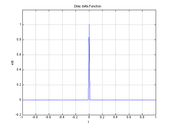
- The delta function
Properties and signal types
Manipulating signals
- time reversal
- time shift
- time dilation/contraction
- Difference btween CT & DT
Composing Signals
Why digital signal processing?
If you're working on a computer, or using a computer to manipulate your data, you're almost-certainly working with digital signals. All manipulations of the data are examples of digital signal processing (for our purpose processing of discrete-time signals as instances of digital signal processing).
Examples of the use of DSP:
- Filtering: Eliminating noise from signals, such as speech signals and other audio data, astronomical data, seismic data, images.
- Synthesis and manipulation: E.g. speech synthesis, music synthesis, graphics.
- Analysis: Seismic data, atmospheric data, stock market analysis.
- Voice communication: processing, encoding and decoding for store and forward.
- Voice, audio and image coding for compression.
- Active noise cancellation: Headphones, mufflers in cars
- Image processing, computer vision
- Computer graphics
- Industrial applications: Vibration analysis, chemical analysis
- Biomed: MRI, Cat scans, imaging, assays, ECGs, EMGs etc.
- Radar, Sonar
- Seismology.
Defining Signals
What is a Signal?
A signal is a way of conveying information. Gestures, semaphores, images, sound, all can be signals.
Technically - a function of time, space, or another observation variable that conveys information
We will disitnguish
3 forms of signals:
- Continuous-Time/Analog Signal
- Discrete-Time Signal
- Digital Signal
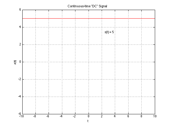
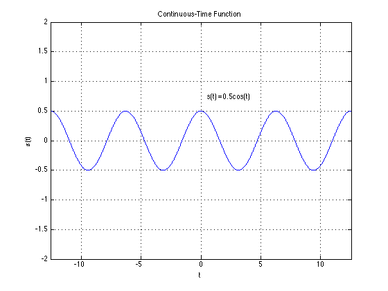
Continuous-time (CT)/Analog Signal
A finite, real-valued, smooth function $s(t)$ of a variable t which usually represents time. Both s and t in $s(t)$ are continuous
Why real-valued?
Usually real-world phenomena are real-valued.
Why finite?
Real-world signals will generally be bounded in energy, simply because there is no infinite source of energy available to us.
Alternately, particularly when they characterize long-term phenomena (e.g. radiation from the sun), they will be bounded in power.
Real-world signals will also be bounded in amplitude -- at no point will their values be infinite.
In order to claim that a signal is “finite”, we need some characterization of its “size”. To claim that the signal is finite is to claim that the size of the signal is bounded -- it never goes to infinity. Below are a few characterizations of the size of a signal. When we say that signals are finite, we imply that the size, as defined by the measurements below is finite.
- The “energy” of a signal characterizes its “size”.
$E=\int_{-\infty}^{\infty}s^2(t)dt$
- The "power" of a signal = energy/unit time
$P=\lim_{T \to \infty} \frac{1}{2T} \int_{-T}^{T} s^2(t)\,dt.$
- Instantaneous power
$P_i = \lim_{\Delta t \to 0} \frac{1}{\Delta t} \int_{t}{t + \Delta t} s^2(\tau),d \tau.$
- Amplitude = $max | s(t)|$
Why smooth?
Real world signals never change abruptly/instananeously. To be more technical, they have finite bandwidth.
Note that although we have made assumptions about signals (finiteness, real, smooth), in the actual analysis and development of signal processing techniques, these considerations are generally ignored.
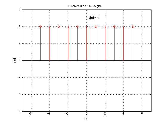
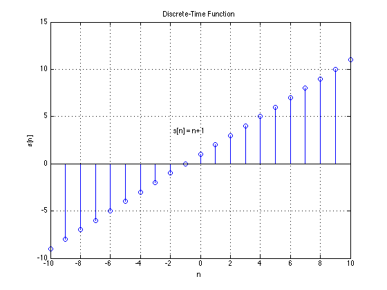
Discrete-time(DT) Signal
A discrete-time signal is a bounded, continuous-valued sequence $s[n]$. Alternately, it may be viewed as a continuous-valued function of a discrete index $n$.
We often refer to the index $n$ as time, since discrete-time signals are frequently obtained by taking snapshots of a continuous-time signal as shown below.
More correctly, though, $n$ is merely an index that represents sequentiality of the numbers in $s[n]$.
If they DT signals are snapshots of real-world signals
realness and
finiteness apply.
Below are several characterizations of size for a DT signal
- Energy
$E=\sum_n s^2[n]$
- Power
$P=\lim_{N \to \infty} \frac{1}{2N+1} \sum_{n=-N}^{N} s^2[n].$
- Amplitude = $max | s[n]|$
Smoothness is not applicable.
Digital Signal
We will work with digital signals but develop theory mainly around discrete-time signals.
Digital computers deal with digital signals, rather than discrete-time signals. A digital signal
is a sequence $s[n]$, where index the values $s[n]$ are not only finite, but can only take a finite set of values. For instance,
in a digital signal, where the individual numbers $s[n]$ are stored using 16 bits integers, $s[n]$ can take one of only 216 values.
In the digital valued series $s[n]$ the values s can only take a fixed set of values.
Digital signals are discrete-time signals obtained after "digitalization." Digital signals too are usually obtained by taking measurements from
real-world phenomena. However, unlike the accepted norm for analog signals, digital signals may take complex values.
Presented above are some criteria for real-world signals.
Theoretical signals are not constrained
real- this is often violated; we work with complex numbers
finite/bounded
energy - violated ALL the time
. Signals that have infinite temporal extent, i.e. which extend from $-\infty$ to $\infty$, can have infinite energy.
power - almost never: nearly all the signals we will encounter have bounded power
smoothness-- this is often violated by many of the continuous time signals we consider.
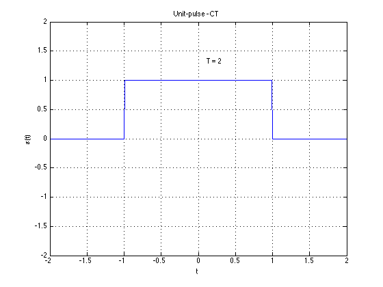
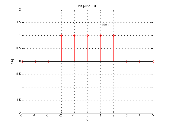
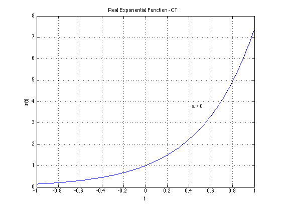
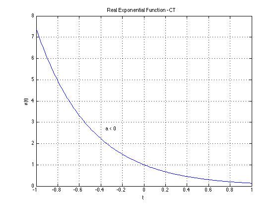
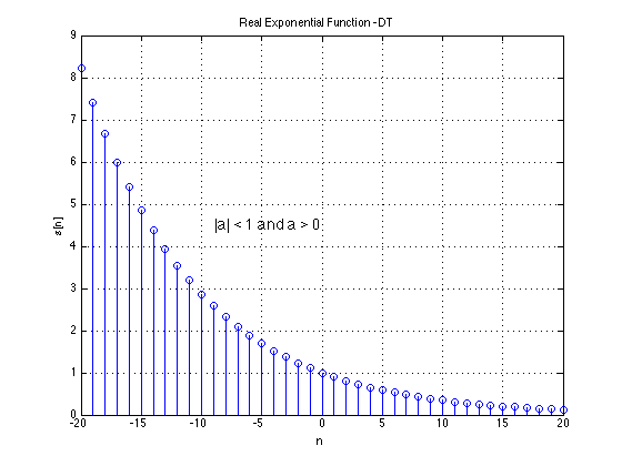
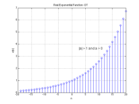
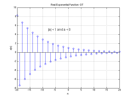
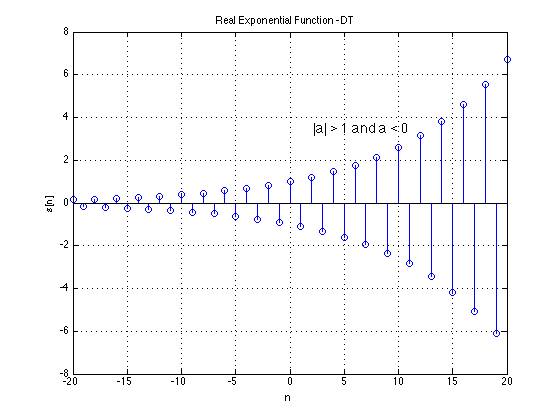
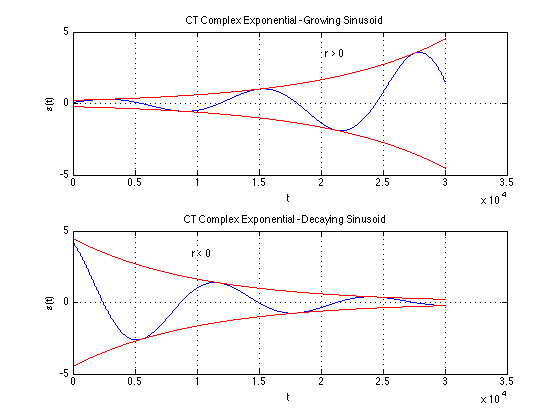
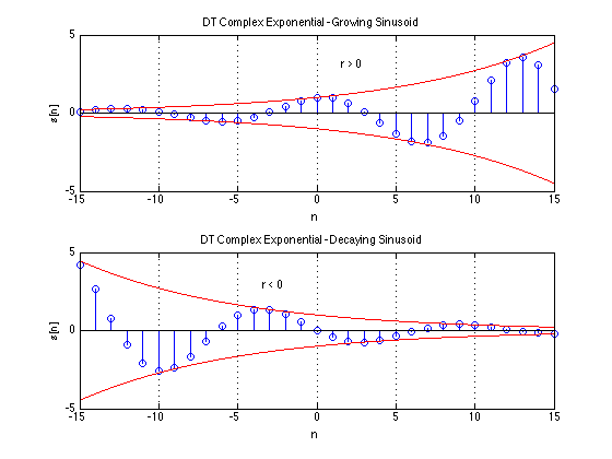
Examples of "Standard" Signals
We list some basic signal types that are frequently encountered in DSP. We list both their continuous-time and discrete-time versions.
Note that the analog continuous-time versions of several of these signals are artificial constructs -- they violate some of the conditions we
stated above for real-world signals and cannot actually be realized.
Signal Types
We can categorize signals by their properties, all of which will affect our analysis of these signals later.
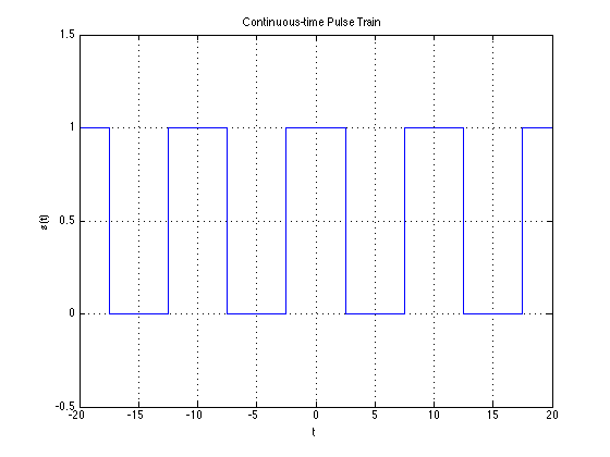
Periodic signals
A signal is periodic if it repeats itself exactly after some period of time. The connotations of periodicity, however, differ for continuous-time and discrete time signals. We will deal with each of these in turn.
Continuous Time Signals
Thus, in continous time a signal if said to be periodic if there exists any value $T$ such that
\[
s(t) = s(t + MT),~~~~~ -\infty\leq M \leq \infty,~~\text{integer}~M
\]
The smallest $T$ for which the above relation holds the period of the signal.
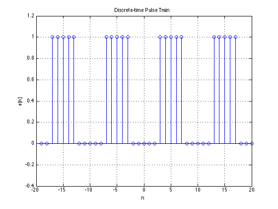
Discrete Time Signals
The definition of periodicity in discrete-time signals is analogous to that for continuous time signals, with one key difference: the period must be an integer. This leads to some non-intuitive conclusions as we shall see.
A discrete time signal $x[n]$ is said to be periodic if there is a positive integer value $N$ such that
\[
x[n] = x[n + MN]
\]
for all integer $M$. The smallest $N$ for which the above holds is the period of the signal.
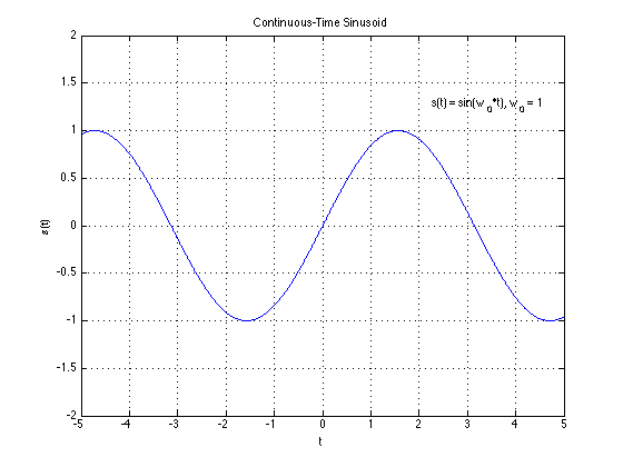
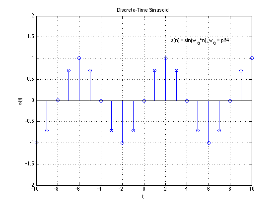
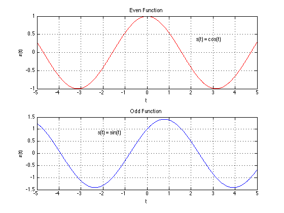
Even and odd signals
An
even symmetic signal is a signal that is mirror reflected at time $t=0$. A signal is even if it has the following property:
\[
\text{Continuous time:}~s(t) = s(-t) \\
\text{Discrete time:}~s[n] = s[-n]
\]
A signal is odd symmetic signal if it has the following property:
\[
\text{Continuous time:}~s(t) = -s(-t) \\
\text{Discrete time:}~s[n] = -s[-n]
\]
The figure below shows examples of even and odd symmetric signals. As an example, the cosine is even symmetric, since $\cos(\theta) = \cos(-\theta)$, leading to $\cos(\omega t) = \cos(\omega(-t))$. On the other hand the sine is odd symmetric, since $\sin(\theta) = -\sin(-\theta)$, leading to $\sin(\omega t) = -\sin(\omega(-t))$.
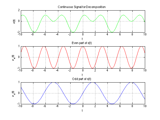
Decomposing a signal into even and odd components
Any signal $x[n]$ can be expressed as the sum of an even signal and an odd signal, as follows
\[
x[n] = x_{even}[n] + x_{odd}[n]
\]
where
\[
x_{even}[n] = 0.5(x[n] + x[-n]) \\
x_{odd}[n] = 0.5(x[n] - x[-n])
\]
Manipulating signals
Signals can be composed by manipulating and combining other signals. We will consider these manipulations briefly.
Scaling
Simply scaling a signal up or down by a gain term.
Continuous time: $y(t)= a x(t)$
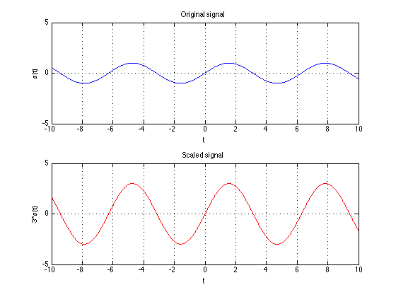
Discrete time: $y[n]= a x[n]$
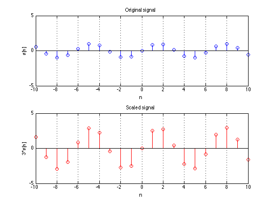
$a$ can be a real/imaginary, positive/negative. When $a is negative, the signal is flipped across the y-axis.
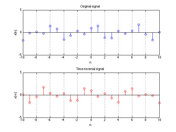
Time reversal
Flipping a signal left to right.
Continuous time: $y(t) = x(-t)$
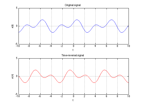
Discrete time: $y[n] = x[-n]$
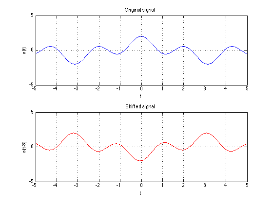
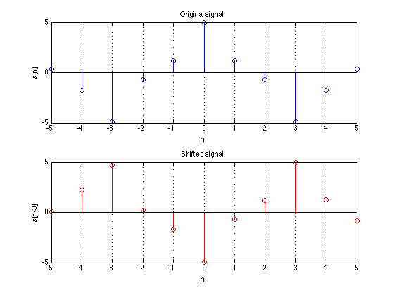
Time shift
The signal is displaced along the indendent axis by $\tau$ (or N for discrete time). If $\tau$ is positive, the signal is delayed and if $\tau$ is
negative the signal is advanced.
Continuous time: $y(t) = x(t- \tau)$
Discrete time: $y[n] = x[n - N]$
Dilation
The time axis itself can scaled by $\alpha$.
Continuous time: $y(t) = x(\alpha t)$
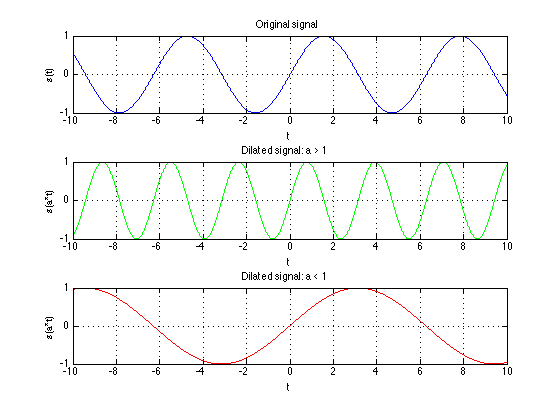
Discrete time: $y[n] = x[/alpha n]$
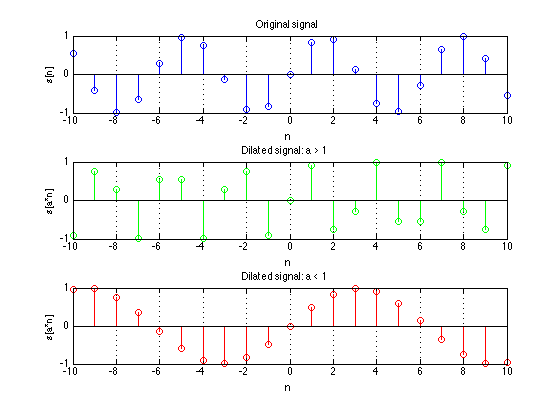
The DT dilation differs from CT dilation because $x[n]$ is ONLY defined at integer n so for $y[n] = x[\alpha n]$ to exist "an" must be an integer.
However $x[\alpha n]$ for $a \neq 1$ loses some samples. You can never recover x[n] fully from it. This process is often called decimincation.
For DT signals
$y[n] = x[\alpha n]$ for $\alpha < 1$ does not exist. Why?
y[0] = x[0] OK
y[1] = x[\alpha] If $a < 1$ this does not exist. Instead we must interpolate zeros for undefined valued if $an$ is not an integer.
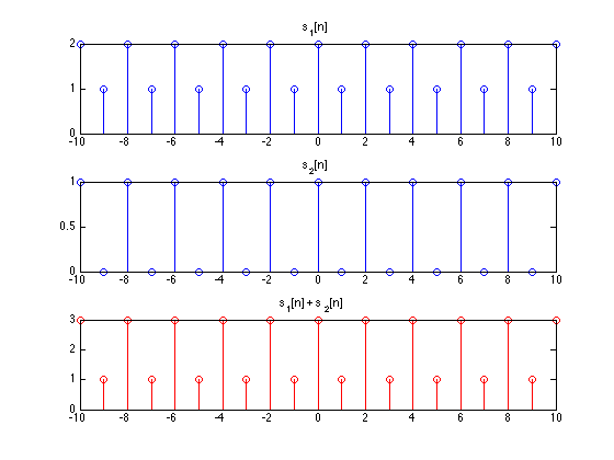
Composing Signals
Signals can be composed by manipuating and combining other signals
There are may ways of combining signals and we consider the following two:
ADDITION
Continuous-time: $y(t) = x_1(t) + x_2(t)$
Discrete-time: $y[n] = x_1[n] + x_2[n]$
MULTIPLICATION
Continuous-time: $y(t) = x_1(t) x_2(t)$
Discrete-time: $y[n] = y_1[n] y_2[n]$
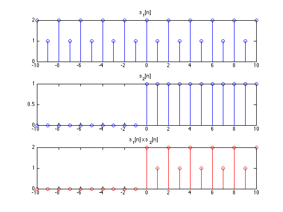
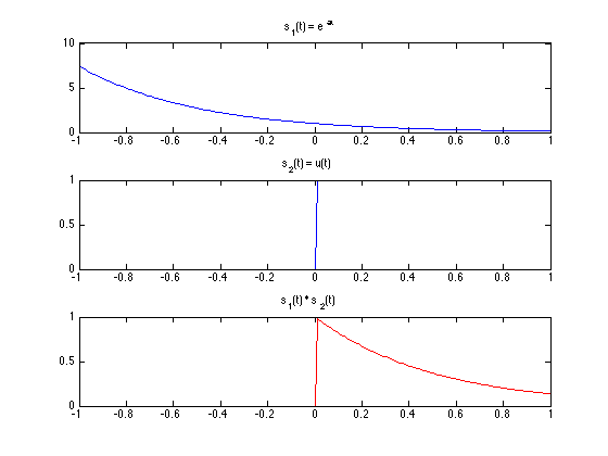
$x_1[n]$ and $x_2[n]$ can themselves be ontained by manipulating other signals. For exmple below we have a truncated expontential begins at t=0.
This signal can be obtained by multiplying
$x_1(t) = e^{\alpha t}$ and $x_2(t) = u(t)$
where $y(t) = e^{\alpha t} u(t)$ for $\alpha < 0$. Same is true for discrete time signals. In genral one-sided signals can be obtained by
multiplying by u[n] (or shifted/time-reversed versions of u[n] or u(t))
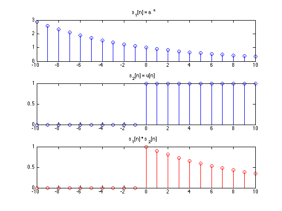
In gernal one-sided signals can be obtained by multiplying by u[n] (or shifted/time-reversed versions of u[n] or u(t)).
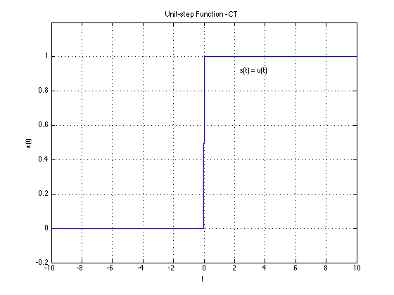
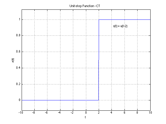
Deriving Basic Signals from One Another
It is possible to derive one signal from another simply through mathematical manipulation. Remember in continuous-time; $u(t)$ and $\delta(t)$
$\delta(t) = \frac{du(t)}{dt}$
$u(t) = \int_{-\infty}^{t} \delta (\tau) d\tau$
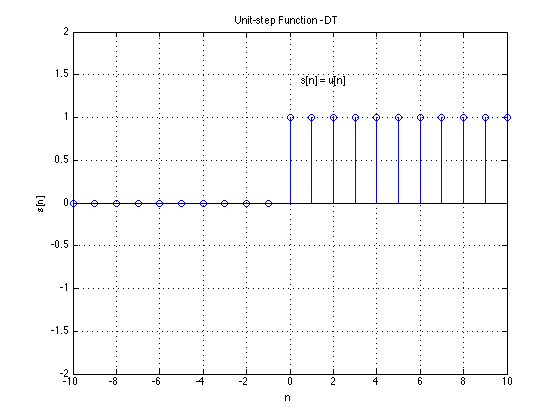
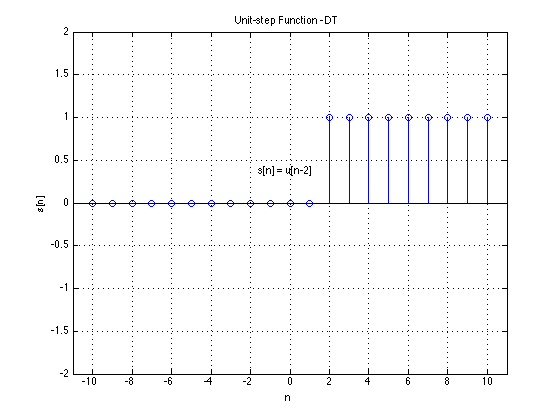
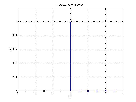
In discrete-time: $u[n]$ and $\delta[n]$
So
$\delta[n] = u[n] - u[n-1]$
$\delta[n] = u[n] - u[n-k]$ and $u[n] = \sum_{k=\infty}^{n} \delta[k]$
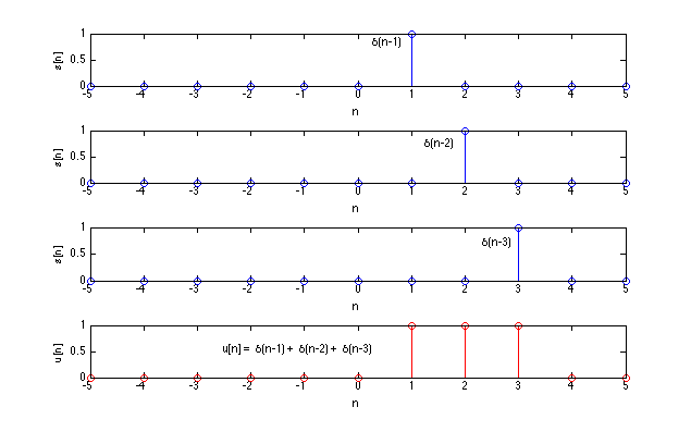
Another way of defining $u[n]$ is
$u[n] = \sum_{k=0}^{\infty}\delta[n-k]$
In general:
$u[n] = \sum_{k= -\infty}^{\infty} u[k]\delta[n-k]$
This concludes the introduction to signals. To review we have discussed the importantance of DSP, types of signals and their properties, manipulation of signals,
and signal composition. Next we will discuss systems.