FOURIER TRANSFORM

• Introduction
• Fourier Series of Pulse Train
• Fourier Transform - Frequency Representation of Periodic Signals
• Fourier Transform Properties
• Conditions for Existence of Fourier Transforms
• Properties of the Fourier transform Cont.
• More examples of Fourier transform

Introduction

We have seen how to compute the frequency composition of periodic signals, now we will consider aperiodic signals.

Recall the Fourier series representation of periodic signals: \[s(t) = \sum_{k = - \infty}^{\infty}C_k e^{\frac{j 2 \pi k t}{T}} = \sum_{k = -\infty}^{\infty} C_k e^{j \omega_o kt}\] \[C_k = \frac{1}{T} \int_{0}^{T}s(t) e^{\frac{-j 2 \pi k}{T}}dt = \frac{\omega_o}{2 \pi} \int_{0}^{T}s(t)e^{-j \omega_o t}dt \text{ where } \omega_o = \frac{2 \pi}{T}\]

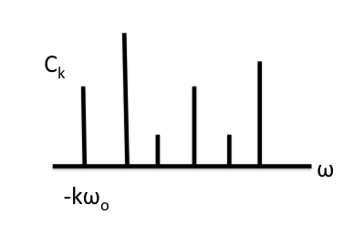
The $C_k$ terms do not tell us anything about the actual compsotion of the signal. If we plot $C_k$ again k we get plot such as:

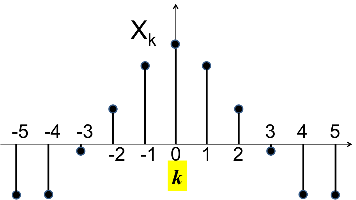
The plot by itself is insufficient to reconstruct s(t). Another key item of information required is T, the period or $\omega_o$, which is the fundemental frequency (in radians/sec).

We can compose completely diifferent signals by simply changing $w_o$ from the same $C_k$ sequence.

Let us instead represent the frequency content slightly differently where the axis is now really the frequency.

Define $C_\omega = C_k$ for $\omega = \frac{2 \pi}{T}k = k \omega_o$

Now our frequency plots become:

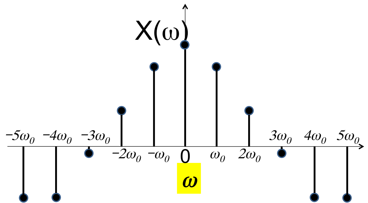
But $C_k$ only tells us what happens at $\omega = \frac{2 \pi}{T}k = k \omega_o$

What is the value of the spectrum at other values of $\omega$?

For this we will use the following: \[ \lim_{T \to \infty} \frac{1}{2T} \int_{-T}^{T}e^{j \omega_1 t} e^{-j \omega_2 t} = \begin{cases} 0, & \omega_1 \neq \omega_2 \\ 1, & \omega_1 = \omega_2 \end{cases} \]

We will not prove this rigorously, but the intuition is easy to see: \[e^{j \omega_1 t} e^{j \omega_2 t} = (cos(\omega_1t) + j sin(\omega_1 t)) (cos(\omega_2t) + j sin(\omega_2))\] \[( cos(\omega_1t)cos(\omega_2t) + sin(\omega_1 t)sin(\omega_2 t) + j(sin(\omega_1 t) cos(\omega_2 t) - cos(\omega_1 t) sin(\omega_2 t) ))\]

We know from our earlier lectures that if $\omega_1 \neq \omega_2$ then $sin(\omega_1 t) sin(\omega_2 t)$ is periodic with both positive and negative components for that within any period canceling themselves out.

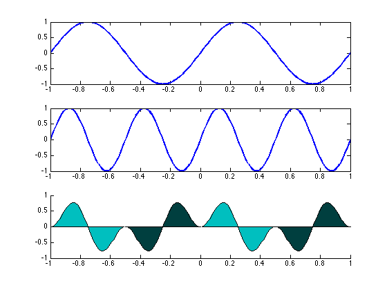
The residual non-zero area is no more than the area in half a period. \[\text{So } \lim_{T \to \infty} \int_{-T}^{T}sin(\omega_1 t)sin(\omega_2 t)dt < \int_{0}^{\frac{T_{period}}{2}}sin(\omega_1 t)sin(\omega_2 t)dt = C\] \[\text{So } \lim_{T \to \infty} \frac{1}{2T} \int_{-T}^{T}sin(\omega_1 t) sin(\omega_2 t)dt < \lim_{T \to \infty} \frac{1}{2T}C = 0\]

This applies to all components of $e^{j \omega_1 t} e^{j \omega_2 t}$

Hence: \[\lim_{T \to \infty} \frac{1}{2T} \int_{-T}^{T}e^{j \omega_1 t} e^{-j \omega_2 t} = 0 \text{ if } \omega_1 \neq \omega_2\]

The value is only define if $\omega_1 = \omega_2$ so for $\omega_1 = \omega_2$: \[\lim_{T \to \infty} \frac{1}{2T} \int_{-T}^{T}e^{j \omega_1 t} e^{-j \omega_2 t} = \lim_{T \to \infty} \frac{1}{2T} \int_{-T}^{T}dt = \frac{2T}{2T} = 1\]

Let's compute $C_\omega$ at $\omega \neq \omega_o k$ for integer k: \[ \begin{align*} C_\omega &= \lim_{N \to \infty} \frac{1}{NT} \int_{-NT}^{NT}s(t)e^{-j \omega t}dt \\ &= \lim_{N \to \infty} \frac{1}{NT} \int_{-\frac{NT}{2}}^{\frac{NT}{2}} \sum_{k = -\infty}^{\infty} C_k e^{j \omega_o kt} e^{-j \omega t}dt \\ &= \sum_{k = -\infty}^{\infty} C_k \lim_{N \to \infty} \frac{1}{NT} \int_{-frac{NT}{2}}^{\frac{NT}{2}} e^{j \omega_o kt} e^{- j \omega t}dt \\ &= 0 \end{align*} \]

$C_\omega$ is 0 at $\omega \neq k \omega_o$ such as at all intermediate values of $\omega$

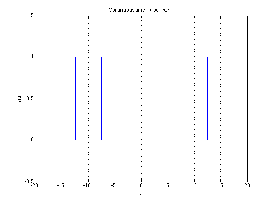
Fourier Series of Pulse Train

Let's revisit the Fourier series of a pulse train:

\[ s(t) = \begin{cases} 1, & 0 \leq |t| < \frac{d}{2} \\ 0, & \frac{d}{2} \leq |t| < \frac{T}{2} \\ s(t +T) \end{cases} \] \[ \begin{align*} s(t) &= \sum_{k = -\infty}^{\infty} C_k e^{\frac{j 2 \pi k t}{T}} \\ &= \sum_{k = -\infty}^{\infty} C_k e^{j w_o kt} \end{align*} \] \[ \begin{align*} C_k &= \frac{sin \frac{\pi k d}{T}}{\pi k} \\ &= \frac{1}{T} \frac{sin \frac{w_o k d}{2}}{\frac{k w_o}{2}} \end{align*} \] \[\omega_o k = \omega \text{ , } C_k \rightarrow C_\omega \] \[T C_\omega = \frac{sin \frac{\omega d}{2}}{(\frac{w}{2})} = \frac{2sin \frac{\omega d}{2}}{\omega}\]

The "spectrum" looks like this

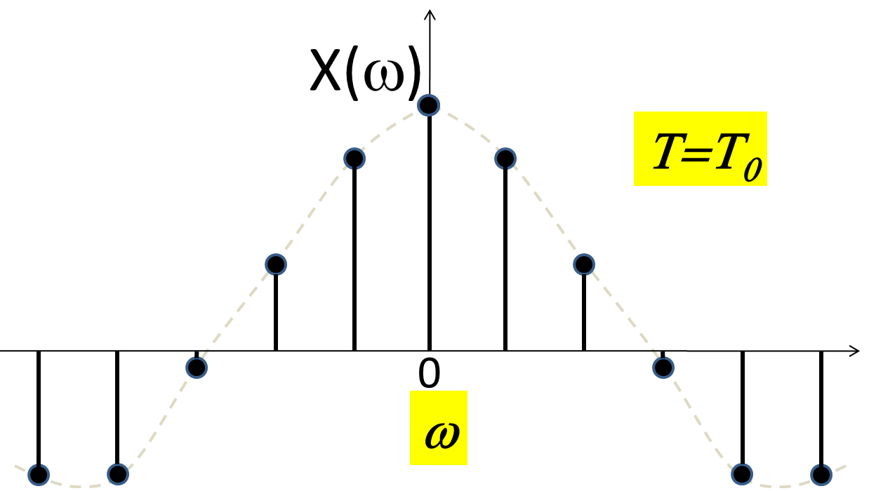
The lines (stem plot) show the actual FS coefficients. They occur only at $\omega = k \omega_o$. At other values of $\omega$ the spectrum is 0.

The continuous line in the figure is the envelope.

The main "lobe" becomes 0 at $\frac{\omega d}{2} = \pi \Rightarrow \omega = \frac{2 \pi}{d}$

and $\frac{\omega d}{2} = -\pi \Rightarrow \omega = \frac{-2 \pi}{d}$

Note that the width of this "lobe" depends ONLY on the width "d" of the pulses in the pulse train, but not on the actual period.

Earlier we showed that for a fixed T the "lobe" & width increases with decreasing "d".

Lets see now what happens with a increasing T for a fixed "d".

As T increases, $\frac{2 \pi}{T} = \omega$ = spacing between the peaks (stems) in the spectrum decreases.

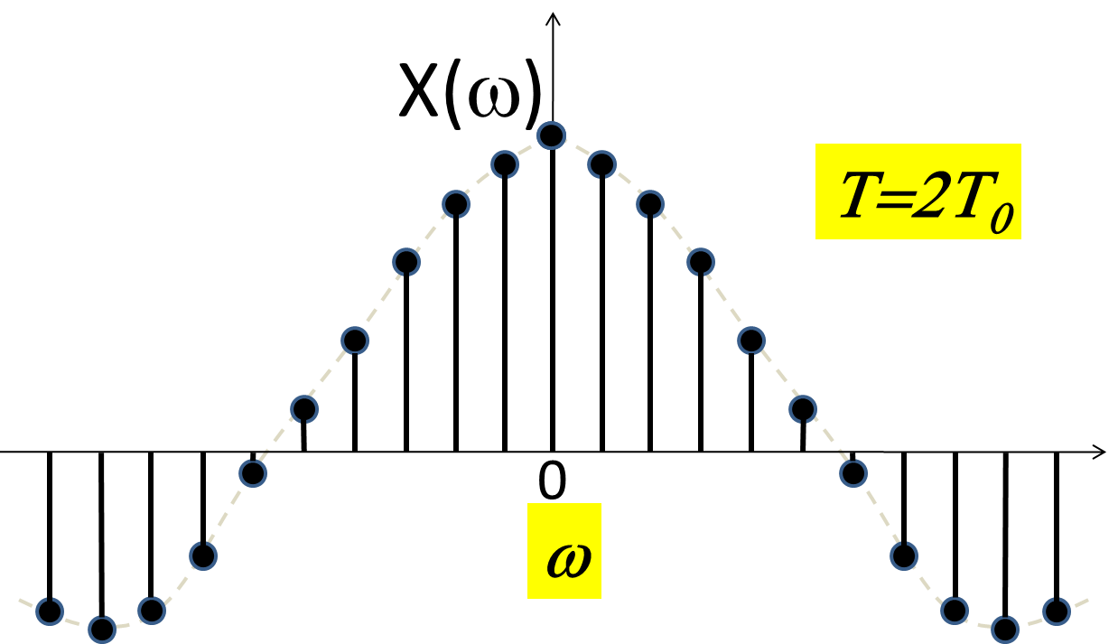
As the period T' between the pulses increases the spacing between the lines in the spectrum.

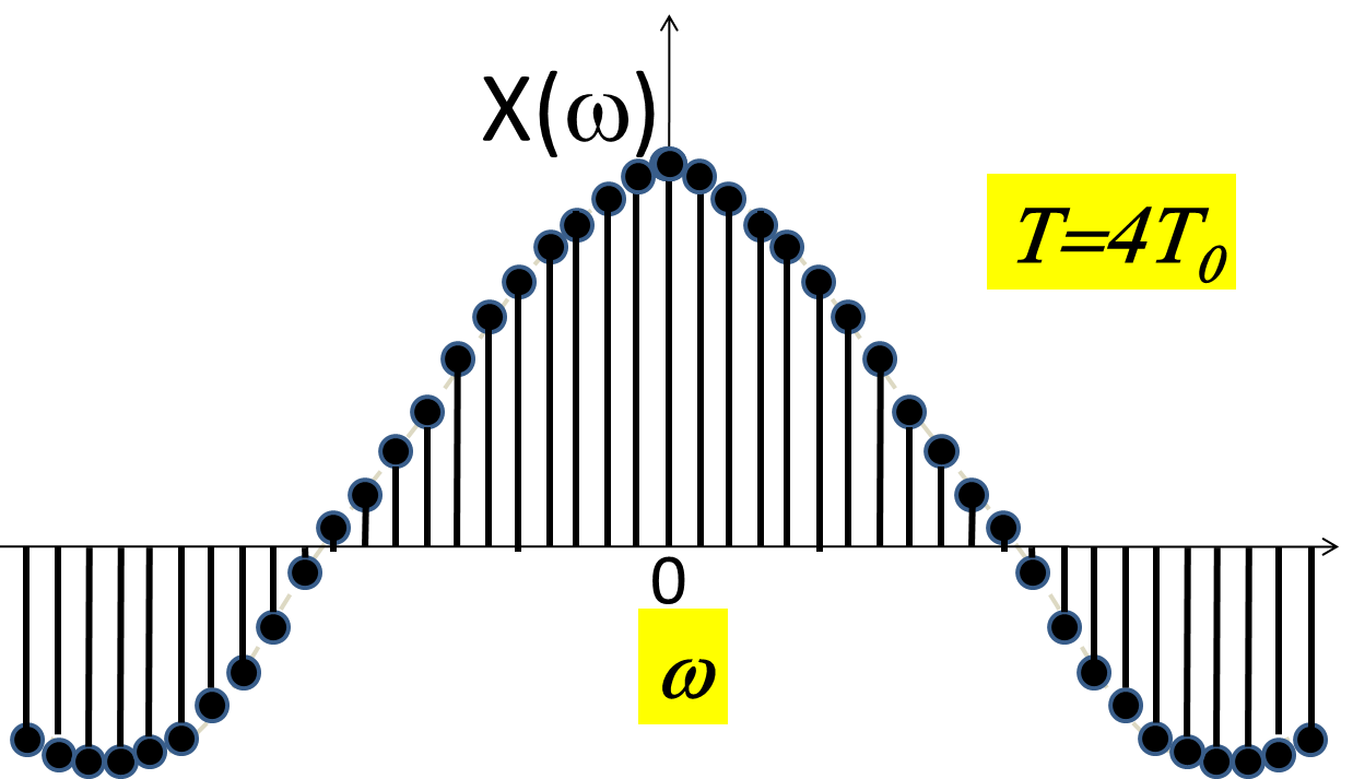
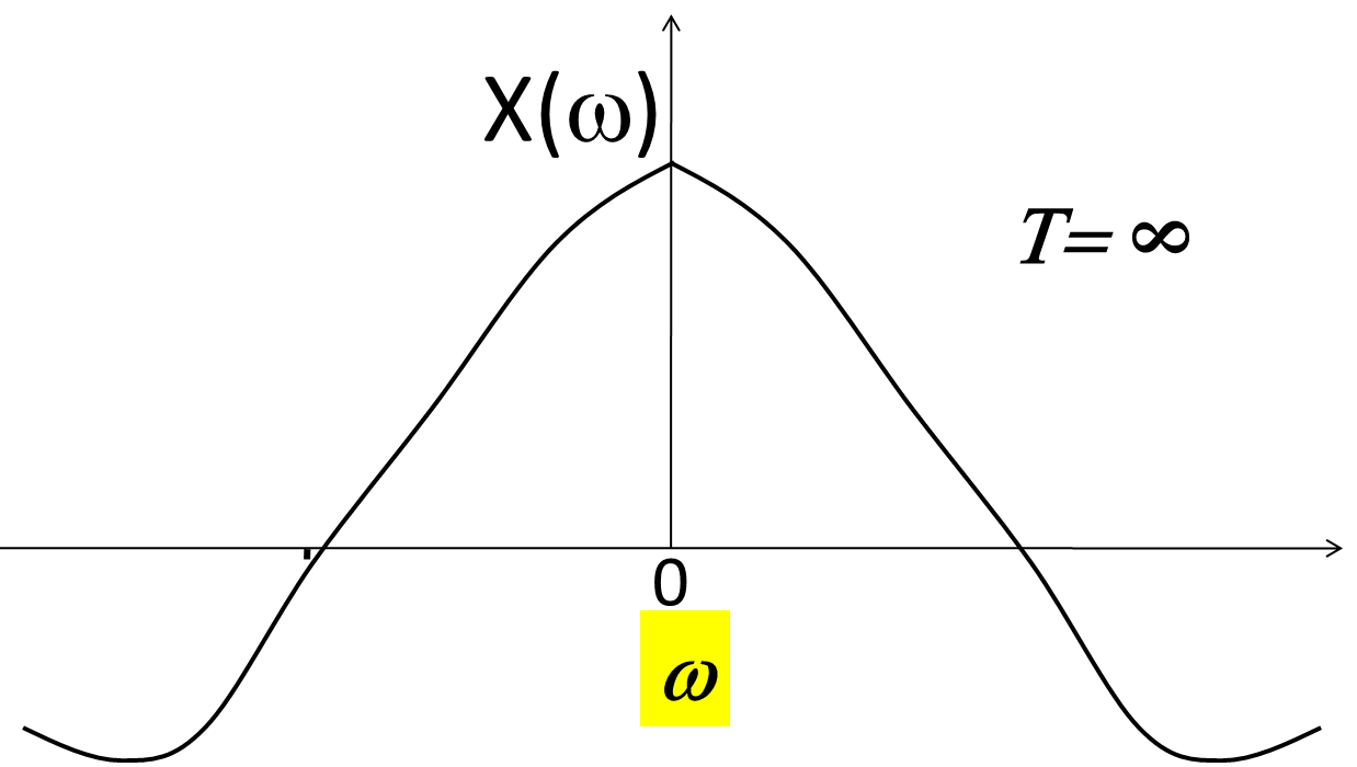
In the limit, as $T' \rightarrow \infty$, we will have only one pulse. This is not a periodic signal -- it has a period of $\infty$. The spectrum on the other hand will become a continuous line as the stem spacing goes to 0

This appears anomalous on the surface. If the spectrum becomes a continuous line, the spacing between stems becomes smaller. More stems in the main lobe would imply more energy within the main lobe. The spectrum seems to show that as the space between the pulses increase the energy of the signal increases!

On the other hand fewer pulses actually implies less energy.

The answer to this conundrum lies in the fact that we actually plotted: \[T_1 a_k = C_\omega \frac{2 \pi}{\omega_o}\]

This is not the spectral value itself -- it actually has the same dimersion as spectrum per unit frequency.

In other words its not the spectrum, but the spectral density!

Let us derive this a bit more formally to make it obvious.

Fourier Transform - Frequency Representation of Periodic Signals

Consider an aperiodic signal $s(t)$

We can now compose an artificial signal $\hat{s}(t)$ that is periodic with T

\[\hat{s}(t) = \begin{cases} s(t), & -b \leq t < a \\ \hat{s}(t+T), & \text{otherwise} \end{cases} \] \[s(t) = \lim_{T \to \infty} \hat{s}(t)\]

As the period increases, eventually we will have only one period of $\hat{s}(t)$, which is $s(t)$

The Fourier Series of $\hat{s}(t)$ is given by:

\[\hat{S}_{\omega} = \begin{cases} \hat{C}_k, & \omega = k \omega_o \\ 0, & otherwise \end{cases} \]

or

\[ \hat{S}_\omega = \begin{cases} \frac{1}{T} \int_{-\frac{T}{2}}^{\frac{T}{2}} s(t) e^{-j \omega t}dt, & \omega = k \frac{2 \pi}{T} \\ 0, & otherwise \end{cases} \]

The spacing between stems are $\frac{2 \pi}{T}$. Let's call this $\Delta \omega$. As $T \rightarrow \infty$, $\Delta \omega \rightarrow 0$

\[S_\omega = \lim_{T \to \infty} \hat{S}_\omega = \lim_{T \to \infty} \frac{1}{T} \int_{-\frac{T}{2}}^{\frac{T}{2}}s(t) e^{-j \omega t}dt\] \[\text{Let } \frac{2 \pi}{T} = \omega\] \[\hat{S}_\omega = \frac{\Delta \omega}{2 \pi} \int_{-\frac{T}{2}}^{\frac{T}{2}}s(t) e^{-j \omega t}dt\] \[\text{Let }\frac{\hat{S}_\omega}{\Delta \omega} = \hat{S}_\omega \text{ , } \frac{S_\omega}{\Delta \omega} = S(\omega)\] \[ \begin{align*} S(\omega) &= \lim_{T \to \infty} \hat{S}(\omega) \\ &= \lim_{\Delta \omega \to 0} \hat{S}(\omega) \end{align*} \] \[\hat{s}(t) = \sum_{k = -\infty}^{\infty} \hat{S}(k \Delta \omega) e^{jk \Delta \omega t}\Delta \omega\] \[\hat{S}(\omega) = \frac{1}{2 \pi} \int_{-\frac{T}{2}}^{\frac{T}{2}}s(t) e^{-j \omega t}dt\]

Lets consider the second equation at any particular $t$

The equation for $\hat{s}(t)$ is simply computing the total area of all the boxes. Each box is $\Delta \omega$ wide. The $k^{th}$ box has a heigh $\hat{s}(k \Delta \omega) e^{kj \Delta \omega t}$ and the area of the $k^{th}$ box is $\hat{s}(k \Delta \omega) e^{kj \Delta \omega t} \Delta \omega$

As $\Delta \omega$ decreases the summation: \[\sum_{k = -\infty}^{\infty} \hat{s}(k \Delta \omega) e^{jk \Delta \omega t}\Delta \omega\] simply becomes the total area under the curve \[\lim_{\Delta \omega \to 0} \sum_{k = -\infty}^{\infty} \hat{s}(k \Delta \omega) e^{jk \Delta \omega t}\Delta \omega = \int_{-\infty}^{\infty}\hat{S}(\omega) e^{j \omega t}d \omega\]

But we have: \[s(t) = \lim_{T \to \infty} \hat{s}(t) = \lim_{\Delta \omega \to 0} \hat{s}(t)\] \[\text{and}\] \[S(\omega) = \lim_{\Delta \omega \to 0} \hat{S}(\omega)\] \[s(t) = \lim_{\Delta \omega \to 0} \hat{s}(t) = \lim_{\Delta \omega \to 0} \sum_{k = -\infty}^{\infty} \hat{S}(k \Delta \omega) e^{j \Delta \omega t} \Delta \omega\] \[ s(t) = \int_{-\infty}^{\infty}S(\omega) e^{j \omega t}d \omega \text{ } (1) \] Returning to: \[\hat{S}(\omega) = \frac{1}{2 \pi} \int_{-\frac{T}{2}}^{\frac{T}{2}}s(t)e^{-j \omega t}dt\] \[S(\omega) = \lim_{T \to \infty} \hat{S}(\omega) = \lim_{T \to \infty} \frac{1}{2 \pi} \int_{-\frac{T}{2}}^{\frac{T}{2}}s(t) e^{-j \omega t}dt\] \[S(\omega) = \frac{1}{2 \pi} \int_{-\infty}^{\infty}s(t) e^{-j \omega t}dt \text{ }(2) \]

Note that $S(\omega) = \lim_{\Delta \omega \to 0} \frac{S_\omega}{\Delta \omega}$

This represents the spectral density at $\omega$. It is a density. The total spectral value in any spectral band $(\omega,\omega + \Delta \omega)$ $\approx S(\omega) \Delta \omega$ for small $\Delta \omega$

The two equations (1) and (2) above are called the Fourier Transform pair of equations.

Equation (2) tells us how to compute the spectral compostion of an aperiodic signal. The outcome $S(\omega)$ is called the Fourier transform of $s(t)$

Equation (1) tells us how to recompose $s(t)$ from its Fourier transform $S(\omega)$

We will represent the computation of the Fourier transform of a signal by the operator FT($\cdot$). We will refer to the computation of the signal from the Fourier tranform as the inverse Fourier tranform and represent it by the operator $\text{FT}^{-1}(\cdot)$: \[S(\omega) = \text{FT}(s(t)) = \frac{1}{2 \pi} \int_{-\infty}^{\infty}s(t)e^{-j \omega t}dt\] \[s(t) = \text{FT}(S(\omega)) = \int_{-\infty}^{\infty} S(\omega) e^{j \omega t}dt\]

It can be easily shown that \[FT^{-1} \cdot FT(s(t)) =s(t)\] \[FT \cdot FT^{-1}(S(\omega)) = S(\omega)\]

Proof: \[FT^{-1} \cdot FT(s(t)) = s(t)\] \[ \begin{align*} LHS &= \frac{1}{2 \pi} \int_{-\infty}^{\infty} S(\omega) e^{j \omega t}dt = \frac{1}{2 \pi} \int_{-\infty}^{\infty} \int_{-\infty}^{\infty} s(t') e^{-j \omega t'}dt e^{j \omega t}dt \\ &= \int_{-\infty}^{\infty}s(t') \left( \frac{1}{2 \pi}\int_{-\infty}^{\infty}e^{-j \omega t'}e^{j \omega t}d \omega \right) dt' \end{align*} \]

We showed ealier that \[\int_{0}^{T}e^{\frac{j2 \pi n_1 t}{T}}e^{\frac{j2 \pi n_2 t}{T}}dt = 0 \text{ for } n_1 \neq n_2\]

A more generic property of the complex expontential is: \[\int_{-\infty}^{\infty} e^{\pm j \omega t}dt = 2 \pi \delta (\omega)\] So: \[\int_{-\infty}^{\infty}e^{-j \omega(t' - t*)}dt = 2 \pi \delta(t' - t^*)\] \[FT^{-1} \cdot FT(s(t)) = \int_{-\infty}^{\infty} s(t') \frac{2 \pi}{2 \pi} \delta(t' -t^*)dt' = s(t)\]

We can similarly show: \[FT \cdot FT^{-1}(S(\omega)) = S(\omega)\]

A note on $2 \pi$: Note we have defined: \[FT\{s(t)\} = S(\omega) = \frac{1}{2 \pi} \int_{-\infty}^{\infty} s(t)e^{-j \omega t}dt\] \[\text{&}\] \[FT^{-1}\{S(\omega)\} = s(t) = \int_{-\infty}^{\infty} S(\omega)e^{j \omega t}d \omega\] For Example: \[FT\{s(t)\} = \frac{1}{\sqrt{2 \pi}} \int_{-\infty}^{\infty} s(t)e^{-j \omega t}dt\] \[\text{&}\] \[FT^{-1}\{S(\omega)\} = \frac{1}{\sqrt{2 \pi}} \int_{-\infty}^{\infty} S(\omega)e^{j \omega t}d \omega\]

As long as the product of the multiplicative constant is $\text{FS}$ & $\text{FS}^{-1}$ goes to $\frac{1}{2 \pi}$, the transform pair remains valid.

Fourier Transform Properties

The Fourier transform is analogous to the Fourier series and has similar properties.

Any signal $s(t)$ can be represented as $s(t) = \int_{-\infty}^{\infty} S(\omega) e^{j \omega t}d \omega$ This representation is unique.

Proof - We have already shown that if we define $S(\omega) = FT\{s(t)\} = \frac{1}{2 \pi} \int_{-\infty}^{\infty} s(t)e^{-j \omega t}dt$ then: \[ \begin{align*} s(t) &= FT^{-1} FT(s(t)) \\ &= FT^{-1}(S(\omega)) \end{align*} \] Hence the representation exists.

Uniqueness: Let there be two difference functions $S_1(\omega)$ and $S_2(\omega)$ such that $s(t) = FT^{-1}(S(\omega)) \text{ & } s(t) = FT(S_(\omega))$ \[s(t) = \int_{-\infty}^{\infty} S_1(\omega)e^{j \omega t}d \omega = \int_{-\infty}^{\infty}S_2(\omega)e^{j \omega t} d \omega\] Multiplying by $e^{-j \omega_1 t}$ and integrating over t \[ \Rightarrow \int_{-\infty}^{\infty}\int_{-\infty}^{\infty}S_1(\omega)e^{j \omega t} e^{- j \omega_1 t}d \omega dt = \int_{-\infty}^{\infty}\int_{-\infty}^{\infty}S_2(\omega)e^{j \omega t} e^{- j \omega_1 t}d \omega dt \] Integrating first with respect to $e^{j \omega t}$ and remembering the orthogonality of $e^{j \omega t}$ \[ \Rightarrow \int_{-\infty}^{\infty}S_1(\omega) \delta(\omega - \omega_1)d \omega = \int_{-\infty}^{\infty}S_2(\omega) \delta(\omega - \omega_1)d \omega \] \[ \Rightarrow S_1(\omega_1) = S_2(\omega_1) \text{ } \forall \omega_1 \]

The representation is unique. QED

Let's now consider other properties of FS that we expect to also see in an DT

1. The spectrum for a tone must have only one frequency
2. The spectrum for a periodic signal should have non-zero values at harmonics of the *incomplete*

Let's check if the above two are true:

1. Spectrum of a Tone \[s(t) = cos(\omega_c t)\] \[ \begin{align*} S(\omega) &= \frac{1}{2 \pi} \int_{-\infty}^{\infty}cos(w_c t)e^{-j \omega t}dt \\ &= \frac{1}{2 \pi} \int_{-\infty}^{\infty} \frac{1}{2} (e^{j \omega_c t} + e^{-j \omega_c t})e^{-j \omega t}dt \\ &= \frac{1}{2 \pi} \left( \frac{1}{2} \int_{-\infty}^{\infty} e^{j(\omega_c - \omega)t}dt + \frac{1}{2} \int_{-\infty}^{\infty}e^{-j(\omega_c +\omega)t}dt \right) \\ &= \frac{1}{2 \pi} \left( \frac{2 \pi}{2} \delta(\omega - \omega_c) + \frac{2 \pi}{2} \delta(\omega + \omega_c)\right) \\ &= \frac{1}{2} \left(\delta(\omega - \omega_c) + \delta(\omega + \omega_c)\right) \end{align*} \]

   

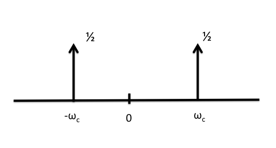
   The FT consists of Dirac delta impulses at $\pm$ the frequency of the cosine.

   The spectrum of a tone has non-zero components only at its frequency

2. Spectrum of a periodic signal

   Let s(t) be periodic with T. We can use the Fourier series to write: \[ \begin{align*} S(\omega) &= \frac{1}{2 \pi} \int_{-\infty}^{\infty}s(t)e^{-j \omega t}dt \\ &= \frac{1}{2 \pi} \int_{-\infty}^{\infty} \sum_{k = -\infty}^{\infty} C_k e^{jk \omega_o t} e^{-j \omega t}dt \\ &= \sum_{k = -\infty}^{\infty} C_k \frac{1}{2 \pi}\int_{-\infty}^{\infty} e^{-j(\omega - k \omega_o)t}dt \\ &= \sum_{k = -\infty}^{\infty} C_k \delta(\omega - k \omega_o) \end{align*} \]

   

   The FT of a periodic signal consists of Dirac deltas at $k \omega_o$ as expected

Conditions for Existence of Fourier Transforms

Fourier Transforms do not actually exist for ALL signals. The signals must satisfy some properties, much like in the case of Fourier series. We refer to these too as Dirichlet's conditions

1. In any finite interval, the signal must have a finite number of extrema
2. In any finite interval it must have a finite number of discontinuities
3. The signal must be absolutely integrable: \[\int_{-\infty}^{\infty}|x(t)|dt < \infty\] This is a "weak" condition ensuring the signal does not blow up which some signals may not satisfy.

A couple of simple examples

1. s(t) = 1 is a constant DC signal \[ \begin{align*} S(\omega) &= \frac{1}{2 \pi} \int_{-\infty}^{\infty} s(t) e^{- j \omega t}dt \\ &= \frac{1}{2 \pi} \int_{-\infty}^{\infty} e^{- j \omega t}dt \\ &= \frac{2 \pi \delta(\omega)}{2 \pi} \\ &= \delta(\omega) \end{align*} \] \[s(t) \longleftrightarrow S(\omega)\] \[1 \longleftrightarrow \delta(\omega)\]
2. $s(t) = \delta(t)$ is a Dirac delta function \[ \begin{align*} S(\omega) &= \frac{1}{2 \pi} \int_{-\infty}^{\infty} \delta(t) e^{-j \omega t}dt \\ &= \frac{1}{2 \pi} \end{align*} \] \[s(t) \longrightarrow S(\omega) \] \[\delta(t) \longrightarrow \frac{1}{2 \pi}\]

   DUALITY

   The Fourier transform of a constant signal is an impulse. The Fourier transform of an impulse is a constant.

   The reason for this symmetry is obvious -- the forward and inverse Fourier transform equations are identical to within a scaling constant ($\frac{1}{2 \pi}$)

   In general if a signal $x(t)$ has a Fourier transform $Y(\omega)$, then a signal $y(t)$ [i.e. a signal that looks like the FT of $x(t)$ but is defined over time] will look like $S(\omega)$

   This symmetry is known as DUALITY

3. $s(t) = \delta(t - T)$ is a shifted impulse \[ \begin{align*} S(\omega) &= \frac{1}{2 \pi} \int_{-\infty}^{\infty} \delta(t-T) e^{-j \omega t}dt \\ &= \frac{1}{2 \pi} e^{-j \omega T} \end{align*} \]

   A shifted impulse transforms to a complex exponential

4. $s(t) = e^{-j \omega_o t}$ is a complex exponential \[ \begin{align*} S(\omega) &= \frac{1}{2 \pi} \int_{-\infty}^{\infty} e^{-j \omega_o T}e^{-j \omega t}dt \\ &= \delta(\omega - \omega_o) \end{align*} \]

   The FT of a commplex exponential signal is a shifted delta (at the frequency of the complex exponetial)

   Once again we see duality: \[e^{j \omega_o t} \rightarrow \delta(\omega - \omega_o)\] \[\delta(t - T) \rightarrow e^{j \omega T} \]

5. $s(t) = e^{-\lambda t}u(t) \text{, } \lambda > 0$ is a one-sided decaying exponential \[ \begin{align*} S(\omega) &= \frac{1}{2 \pi} \int_{0}^{\infty} e^{-\lambda t}e^{-j \omega t}dt \\ &= -\frac{1}{2 \pi(\lambda + j \omega)} \left[e^{-(\lambda + j \omega)t} \right]_{0}^{\infty} \\ &= \frac{1}{2 \pi (\lambda + j \omega)} \end{align*} \]
6. What is the FT of $s(t) = \frac{1}{\lambda + jt}$? Hint: Remember the principle of duality.
7. $s(t) = u(t)$

   This is a decpetiviely simple-looking problem which is actually very complex.

   The answer is: \[ \delta(\omega) = \begin{cases} \frac{\delta(\omega)}{2}, & \omega = 0 \\ \frac{1}{j 2 \pi \omega}, & \omega \neq 0 \end{cases} \] \[\text{or}\] \[\frac{\delta(\omega)}{2} + \frac{1}{j 2 \pi \omega}] \]

   Note that we cannot get this directly from the answer for number (5) by setting $\lambda = 0$ because that result is not defined at $\omega = 0$

   Also note $u(t)$ is not absolutely integreable

Properties of the Fourier transform Cont.

All of the properties are easily proved (if not, the proofs will be provided)

1. Existence & Uniqueness \[\text{FT}(\text{FT}^{-1}(S(\omega))) = S(\omega)\] \[\text{FT}(\text{FT}^{-1}(s(t))) = s(t)\]
2. Linearity \[\text{FT}(a x(t) + b y(t)) = a \text{FT}(x(t)) + b \text{FT}(y(t))\]

3. For real signals $s(t)$, their Fourier transform $S(\omega)$ has the following properly \[S(\omega) = S^*(\omega)\]

   Proof

   For real signal $s(t) = s^*(t)$: \[s(t) = \int_{-\infty}^{\infty} S(\omega) e^{j \omega t}d \omega\] \[ \begin{align*} s^*(t) &= \left( \int_{-\infty}^{\infty}S(\omega)e^{j \omega t}d \omega \right)^* \\ &= \int_{-\infty}^{\infty} S^*(\omega) e^{-j \omega t}d \omega \end{align*} \] \[\text{setting } \omega' = -\omega \text{ , } d \omega = -d \omega'\] \[s^*(t) = \int_{\infty}^{-\infty}S^*(-\omega ')e^{j \omega ' t}(-d \omega ')\] \[s(t) = s^*(t)\] \[ \int_{-\infty}^{\infty}S(\omega)e^{j \omega t}d \omega = \int_{=\infty}^{\infty} S^*(-\omega)e^{k \omega t}d \omega \\ \] \[S(\omega) = S^*(-\omega)\]

   This implies that:

   Real $S(\omega) + j \text{ Imag } S(\omega) = Real S(-\omega) - j \text{ Imag } S(-\omega)$

   Real $S(\omega)$ is even and Imag $S(\omega)$ is odd if $s(t)$ is real

4. Time-shift \[s(t) \longleftrightarrow S(\omega)\] \[s(t - T) \longleftrightarrow S(\omega) e^{-k \omega T}\] Proof \[S(\omega) = \frac{1}{2 \pi} \int_{-\infty}^{\infty} s(t)e^{-j \omega t}dt\] \[s(t - T) \longleftrightarrow \frac{1}{2 \pi} \int_{-\infty}^{\infty} s(t-T)e^{-j \omega t}dt\] \[\text{Let } t' = t-T \text{, } dt' = dt \text{, } t = t' + T\] \[ \begin{align*} s(t - T) &= \frac{1}{2 \pi} \int_{-\infty}^{\infty} s(t')e^{-j \omega (t' + T)}dt' \\ &= e^{-j \omega T} \int_{-\infty}^{\infty} s(t) e^{-j \omega t'} dt'\\ &= S(\omega) e^{-k \omega T} \end{align*} \]
5. Frequency shift \[s(t) \longleftrightarrow S(\omega)\] \[s(t)e^{j \Omega t} \longleftrightarrow s(\omega - \Omega)\] Proof \[ \begin{align*} \text{FT}^{-1}(S(\omega - \Omega)) &= \int_{-\infty}^{\infty}S(\omega - \Omega)e^{j \omega t}d \omega\\ \text{Setting } \omega' = \omega - \Omega \text{, } \omega = \omega' + \Omega \\ &= \int_{-\infty}^{\infty}S(\omega ')e^{j(\omega ' + \Omega)t}D \omega \\ &= e^{j \Omega t} \int_{-\infty}^{\infty}S(\omega ') e^{j \omega ' t}d \omega ' &= e^{j \Omega t}s(t) \end{align*} \]

   This is an instance of the so called modulation property. To shift the frequencies in a signal by $\Omega$, you only have to multiply it by $e^{j \Omega t}$

6. Time scaling \[s(t) \longleftrightarrow S(\omega)\] \[s(\alpha t) \longleftrightarrow \frac{1}{|\alpha|}s(\frac{\omega}{2})\] Proof \[FT(s(\alpha t)) = \frac{1}{2 \pi} \int_{-\infty}^{\infty} s(\alpha t)e^{-j \omega t}dt\] \[\text{Let } t' = \alpha t \text{, } dt = \frac{dt'}{/alpha} \text{, } t = \frac{t'}{\alpha}\] \[s(\alpha t) \longleftrightarrow \frac{1}{2 \pi} \int_{-\infty}^{\infty} s(t')e^{-j \frac{\omega}{\alpha} t'}\frac{dt'}{\alpha}\] \[ \begin{align*} \text{For } \alpha > 0 \text{, } S(\alpha t) &= \left( \frac{1}{2 \pi} \int-{-\infty}^{\infty} s(t')e^{-j \frac{\omega}{\alpha} t'}dt' \right)\frac{1}{\alpha} \\ &= \frac{S(\frac{\omega}{\alpha})}{|\alpha|} \end{align*} \] \[\text{For } \alpha < 0 \begin{cases} t \rightarrow \infty \Rightarrow \alpha t \rightarrow -\infty \\ t \rightarrow -\infty \Rightarrow \alpha t \rightarrow \alpha \end{cases} \]

   Now the limits of the integral

   \[S(\alpha t) \leftrightarrow \left( \frac{1}{2 \pi} \int_{\infty}^{-\infty} s(t')e^{-j \frac{\omega}{\alpha} t'}dt' \right)\frac{1}{\alpha} \]

   Flipping the limits of the integral

   \[ \begin{align*} S(\alpha t) &= \left( -\frac{1}{2 \pi} \int_{\infty}^{-\infty} s(t')e^{-j \frac{\omega}{\alpha} t'}dt' \right)\frac{1}{\alpha} \\ &= - \frac{S(\frac{\omega}{\alpha})}{\alpha} \\ &= \frac{S(\frac{\omega}{\alpha})}{|\alpha|} \end{align*} \] \[s(\alpha t) \longleftrightarrow \frac{S(\frac{\omega}{\alpha})}{|alpha|} \text{ for all } \alpha \neq 0\]
7. Derivatives \[s(t) \longleftrightarrow S(\omega)\] \[\frac{d s(t)}{dt} \longleftrightarrow j \omega S(\omega)\] Proof \[s(t) = \int_{-\infty}^{\infty}S(\omega)e^{j \omega t}d \omega\]

   Differentiating both sides dt:

   \[\frac{d s(t)}{dt} = \int_{-\infty}^{\infty}j \omega S(\omega) e^{j \omega t}dt\] \[\frac{d s(t)}{dt } \longleftrightarrow j \omega S(\omega)\]

   Differentiating in time = multiplying by frequency

   By the duality principle we will find that multiply the signal by time $\longleftrightarrow$ differentiation of the FT

8. Integration \[\int_{-\infty}^{\infty}s(\hat{t})d \hat{t} \longleftrightarrow \frac{S(\omega)}{j \omega} + 2 \pi \delta(\omega)\] Proof \[s(\hat{t}) = \int_{-\infty}^{\infty} S(\omega)e^{j \omega \hat{t}}d \omega\]

   Integrating with respect to $\hat{t}$

   \[ \begin{align*} \int_{-\infty}^{t} s(\hat{t})d \hat{t} &= \int_{-\infty}^{\infty}\int_{-\infty}^{t} S(\omega)e^{j \omega \hat{t}}d \omega \\ &= \int_{-\infty}^{\infty} S(\omega) \frac{e^{j \omega t}}{j \omega}d \omega \\ &= \int_{-\infty}^{\infty}(\frac{S(\omega)}{j \omega})e^{j \omega t} d \omega \end{align*} \] \[\int_{-\infty}^{t}s(\hat{t})d \hat{t} \longleftrightarrow \frac{S(\omega)}{j \omega}\]

   This proof is incorrect. The actualy proof is more detailed & the true property is given by the equation above

   "C" is a constant where $C = \int_{-\infty}^{\infty}s(t)dt$

   If the envelop value of is $s(t) = 0$ then $C = 0$

   The reason for the extra $\delta(\omega)$ term is because even if $s(t)$ is absolutely integrable, $y(t) = \int_{-\infty}^{t}s(t')dt'$ will often not be absolutely integrable.

9. The Product of Two Signals \[\text{Let } x(t) \longleftrightarrow X(\omega) \text{ , } y(t) \longleftrightarrow Y(\omega)\] \[x(t) * y(t) \longleftrightarrow \int_{-\infty}^{\infty}X(\Omega)Y(\omega - \Omega)d \Omega\] Proof \[ \begin{align*} x(t) * y(t) &= \frac{1}{2 \pi} \int_{-\infty}^{\infty}x(t)y(t)e^{-j \omega t}dt \\ &= \frac{1}{2 \pi} \int_{-\infty}^{\infty} \left( \int_{-\infty}^{\infty}(X(\Omega)e^{j \Omega t}d \Omega) \right) y(t)e^{-j \omega t}dt \\ &= \int_{-\infty}^{\infty} X(\Omega) \left( \frac{1}{2 \pi} \int_{-\infty}^{\infty} y(t) e^{-j(\omega - \Omega)t}dt \right) d \Omega \\ &= \int_{-\infty}^{\infty}X(\Omega) Y(\omega - \Omega )d \Omega \end{align*} \]

   When two signals are multiplies in time, their spectra get convolved!

   This is the "modulation" property. When you "modulate" $x(t)$ by $y(t)$ their spectra are convolved.

   \[\text{Let } x(t) \longleftrightarrow X(\omega)\] \[y(t) = cos(w_ot) \longleftrightarrow \frac{1}{2}[\delta(\omega - \omega_o) - \delta(\omega + \omega_o)]\]

   So $x(t)*y(t)$ is a cosine amplitude modulated $x(t)$

   \[\frac{1}{2}(x(\omega - \omega_o) + x(\omega + \omega_o))\]
10. The Convolution Property \[\text{Let } z(t) = \int_{-\infty}^{\infty}x(T)y(t - T)dT = x(t)* y(t)\] \[z(t) \longleftrightarrow 2 \pi X(\omega) Y(\omega)\] Proof \[ \begin{align*} \text{FT}(z(t)) &= \frac{1}{2 \pi} \int_{-\infty}^{\infty}z(t)e^{-j \omega t}dt \\ \frac{1}{2 \pi} \int_{-\infty}^{\infty} \int_{-\infty}^{\infty} x(T)y(t-T)dT e^{-j \omega t}dt \end{align*} \] \[\text{Let } t=T = t' \text{ , } dt = dt' \text{ , } t = t' + T\] \[ \begin{align*} z(t) &\leftrightarrow \frac{1}{2 \pi} \int_{-\infty}^{\infty}x(T)y(t') e^{-j \omega(t' + T)}dTdt' \\ &= \int_{-\infty}^{\infty}x(T)e^{-j \omega T}\left(\frac{1}{2 \pi} \int_{-\infty}^{\infty} y(t')e^{-j \omega t'}dt'\right)dT \\ &= 2 \pi \left((\frac{1}{2 \pi})Y(\omega) \int_{-\infty}^{\infty}x(T)e^{- j \omega T}dT\right) \\ &= 2 \pi Y(\omega) X(\omega) \end{align*} \]

    The transform of the convolution of two signals is the product of their individual Fourier transforms

    This is the most important property we use!

11. Energy Conversation - Parseval's Theorem \[\int_{-\infty}^{\infty}|x(t)|^2dt = 2 \pi \int_{-\infty}^{\infty}|X(\Omega)|^2 d \Omega\] Proof

    In the modulation property let $y(t) = x*(t)$

    Property

    \[x(t) \leftrightarrow X(\omega) \Rightarrow x*(t) \leftrightarrow X*(-\omega)\] \[x(t)x*(t) \leftrightarrow \int_{-\infty}^{\infty}x{\Omega}x*(\Omega - \omega)d \Omega\]

    In general if:

    \[z(t) \leftrightarrow Z(\omega)\] \[ \begin{align*} \int_{-\infty}^{\infty}z(t)dt &= 2 \pi \frac{1}{2 \pi} \int_{-\infty}^{\infty}z(t)e^{-j(0)t}dt \\ &= 2 \pi Z(\omega) \text{\omega = 0} \end{align*} \]

    Applying it to $z(t) = x(t)x*(t)$

    \[ \begin{align*} \int_{-\infty}^{\infty}x(t)x*(t)dt &= \\ &= \int_{-\infty}^{\infty}|x(t)|^2dt \\ &= \int_{-\infty}^{\infty} x(\Omega)x(\omega - \Omega)d\Omega \\ &= 2 \pi \int_{-\infty}^{\infty} |x(\Omega)|^2d \Omega \end{align*} \]

    The area under the square of the signal (i.e. the energy of the signal) = the "energy" of the FT to within $2 \pi$

More examples of Fourier transform

1. What is the Fourier Transform of $s(t) = cos(\omega_o t)$

   Remember: \[cos(\omega_o t) = \frac{1}{2}(e^{j \omega_o t } + e^{-j \omega_o t})\] \[\text{So:}\] \[S(\omega) = \frac{\delta(\omega - \omega_o)}{2} + \frac{\delta(\omega + \omega_o)}{2}\]

   We are using the linearity property here.

2. The Dirac combination: \[s(t) = \sum_{k = -\infty}^{\infty} \delta(t - kT)\] for a periodic signal we can write: \[s(t) = \sum_{k = -\infty}^{\infty} a_k e^{-j \omega_o kt}\] \[ \begin{align*} a_k &= \frac{1}{T} \int_{0}^{T}s(t)e^{j \omega_o kt}dt \\ &= \frac{1}{T} \int_{0}^{T} \delta(t) e^{jk \omega_o t}dt \\ &= e^{jk \omega_o 0} \\ &= 1 \end{align*} \] \[s(t) = \sum_{k = -\infty}^{\infty}e^{-j \omega_o kt}\]

   Observation 1 --> The sum of a harmonically sperated complex exponentials is a pulse train

   \[ \begin{align*} S(\omega) &= FT(s(t)) \\ &= \sum_{k = -\infty}^{\infty} FT(e^{-j \omega_o k t}) \\ &= \sum_{k = -\infty}^{\infty} \delta(\omega - \omega_o k) \end{align*} \]

   The FT of a pulse train is a pulse train. As the spacing in time increases, spacing in frequency decreases.

   Time shift and and linearity properties used in the above example

3. What is the Fourier Transform of: \[cos(\omega_o (t-T))\] Remember: \[cos(\omega_o t) = \frac{1}{2}(delta(\omega - \omega_o) + \delta(\omega + \omega_o))\] Using the shift property: \[cos(\omega_o (t-T)) = \frac{1}{2}(delta(\omega - \omega_o) + \delta(\omega + \omega_o)) e^{-j \omega T}\] \[S(\omega) = \frac{e^{j \omega_o t}}{2} (\delta(\omega - \omega_o) + \delta(\omega + \omega_o))\]
4. What is the Fourier Transform of: \[ s(t) = \begin{cases} 1, & 0 \leq t < T \\ 0, & else \end{cases} \] We can write: \[s(t) = u(t) - u(t - T)\] \[u(t) \rightarrow \frac{1}{j 2 \pi \omega} + \frac{\delta(\omega)}{2}\] \[ \begin{align*} u(t - T) & \rightarrow \frac{e^{-j \omega T}}{j 2 \pi \omega} + \frac{\delta(\omega)}{2} e^{- j \omega T} \\ &= \frac{e^{-j \omega T}}{j 2 \pi \omega} + \frac{\delta(\omega)}{2} \end{align*} \] \[FT(s(t)) = \frac{1}{j 2 \pi \omega} + \frac{\delta(\omega)}{2} - \frac{e^{-j \omega T}}{j 2 \pi \omega} - \frac{\delta(\omega)}{2}\] \[S(\omega) = \frac{1 - e^{-j \omega T}}{j 2 \pi \omega}\] We can re-write this as: \[S(\omega) = e^{\frac{-j \omega T}{2}} (\frac{e^{\frac{j \omega T}{2}}-e^{-\frac{j \omega T}{2}}}{2 j \pi \omega})\] \[e^{-\frac{j \omega T}{2}} \frac{sin \omega T}{\pi \omega}\]
5. What is the Fourier Transform of a centered pulse? Note that this is the same signal as Example 4, but shifted left by $\frac{T}{2}$ Let: \[s_4(t) = \begin{cases} 1, & 0 \leq |t| < \frac{T}{2} \\ 0, & else \end{cases} \] \[s(t) = s_4(t + \frac{T}{2})\] \[ \begin{align*} S(\omega) &= s_4(\omega) e^{\frac{j \omega T}{2}} \\ &= e^{-\frac{j \omega T}{2}} \frac{sin \omega T}{\pi \omega} e^{\frac{j \omega T}{2}} \\ &= \frac{sin \omega T}{\pi \omega} \end{align*} \]
6. What is the Fourier Tranform of: \[ s(t) = \begin{cases} 0, & t < -\frac{T}{2} \\ \frac{2}{T}(t + \frac{T}{2}), & -\frac{T}{2} \leq t < 0 \\ 1 - \frac{2}{T}t, & 0 \leq t \frac{T}{2} \\ 0, & else \end{cases} \] This by itself is tedious to evaluate but we can simply it by writing: \[ s_{diff}(t) = \frac{d s(t)}{dt} \] \[ s_{diff}(t) = \begin{cases} 0, & t < -\frac{T}{2} \\ \frac{2}{T}, & -\frac{T}{2} \leq t < 0 \\ \frac{2}{T}, & 0 \leq t \frac{T}{2} \\ 0, & else \end{cases} \] \[ s_{diff}(t) = \frac{2}{T} u(t + \frac{T}{2}) - \frac{4}{T}u(t) + \frac{2}{T} u(t + \frac{T}{2})\] \[ \begin{align*} S_{diff}(\omega) &= \frac{2}{T} (\frac{e^{\frac{j \omega T}{2}}}{j 2 \pi \omega} + \frac{e^{\frac{j \omega T}{2}}}{2} \delta(\omega)) - \frac{\omega}{T} (\frac{1}{j 2 \pi \omega} + \frac{\delta(\omega)}{2}) + \frac{2}{T} (\frac{e^{-\frac{j \omega T}{2}}}{j 2 \pi \omega} + \frac{e^{-\frac{j \omega T}{2}}\delta(\omega)}{2}) \\ &= \frac{2}{T} \frac{e^{\frac{j \omega T}{2}}}{2 \pi j \omega} + \frac{2}{T} \delta(\omega) - \frac{4}{T} \frac{1}{2 \pi j \omega} - \frac{4}{T} \delta(\omega) + \frac{2}{T} \frac{e^{-\frac{j \omega T}{2}}}{2 \pi j \omega} + \frac{2}{T} \delta(\omega) \\ &= \frac{2}{j T \omega \pi} [cos \frac{\omega T}{2} - 1] \end{align*} \]

   Using the integral property

   \[s(t) = \int_{-\infty}^{T} s_{diff}(t)dt\] \[S(\omega) = \frac{s_{diff}(\omega)}{j \omega} + 2 \pi C \delta(\omega)\] \[C = \int_{-\infty}^{\infty}s_{diff}(t)dt = 0\] \[S(\omega) = \frac{2(1 - cos \omega \frac{T}{2})}{T \pi \omega^2}\]