General Signal Analysis
We now begin discussing how we can represent signals in terms of other signals.
In differential calculus, which most of us are familiar with, we usually work with smooth signals. For such functions we have ways of expressing the signal
in terms of other signals, i.e. a Taylor Series expansion.
- Really close to any $t_o$, the value at the signal can be found if the slope or first derivative $\frac{d(x)}{dt}$ at $t_o$ is known
\[x(t) \approx x(t_0) + x'(t_o)(t-t_o)\]
- Slightly farther away you also need the second derivatirve $\frac{d^2(x)}{dt^2}$
\[x(t) \approx x(t_o) + x'(t_o)(t-t_o) +\frac{x''(t_o)}{2}(t-t_0)^2\]
- Even farther away you need $\frac{d^3(x)}{dt^3}$
\[x(t) \approx x(t_o) + x'(t_o)(t-t_o)+\frac{x''(t_o)}{2}(t-t_o)^2+\frac{x'''(t_o)}{6}(t-t_o)^3\]
In the general case $x(t)$ can be expressed as sum of polynomials:
\[x(t) = x(t_o) + \sum_{k=1}^{\infty} \frac{d^kx(t_o)}{dt^k}(t-t_o)^k\]
Knowing all the derivatives at one time is sufficient to know the signal at all times even if you do not known the exact form of $x(t)$.
For example the set of derivatives:
\[{\frac{d^kx(t)}{dt^k}}\bigg|_{t=t_0} \forall k \geq 0\]
is an alternative but complete representation of x(t). The set of derivatives at any $t_o$ is a transformed representation of $x(t)$.
Back
Signal Processing
In signal processing we often deal with similar transformed representations that tell us all there is to know of a signal $x(t)$, and sometimes
provide intuitions that are not available from inspectoin of $x(t)$ itself.
These repsentations will not be in terms of derivative and polynomials, but other functions with useful properties. One such very important transform
representation is the SPECTRUM.
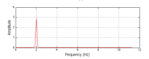
Consider a sinusoid of frequency $f_o$. It can be represented in two ways:
-
As a time signal:
\[x(t) = Asin(2\pi f_ot)\]
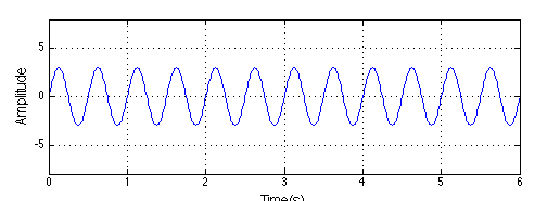
-
As an indicator that simply specifies the frequency and amplitude of the signal.
\[s(t)= \begin{cases}
A, & f = f_o \\
0, & f \neq f_o
\end{cases}
\]
Note that the two representations are strictly
equivalent and both are sufficient to compose the signal. The only extra information required by the second
representation is that the signal is a sinusoid wave.
Consider a signal that is a mixture of two sines:
\[x(t)=asin(2 \pi f_o t)+bsin(2 \pi f_1 t)\]
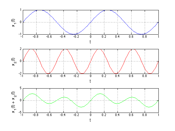
This is a more complex working signal, but it twoo is fully represented by the following notation:
\[s(t)=\begin{cases}
a, & f = f_o \\
b, & f = f_1 \\
0, & otherwise
\end{cases}\]
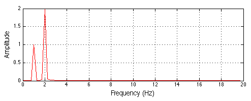
This signal has two frequencies.
We can add more & more frequencies. As we add more frequencies, the signal gets more complex.
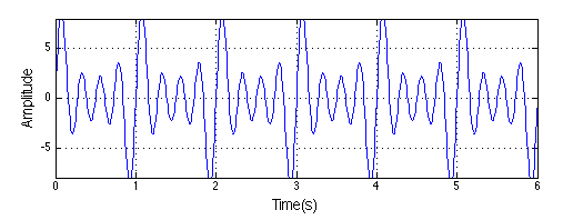
In the limit the frequencies are not discrete but will form a continuum. The composed signal can be surprising.
For example:
\[rect\left(\frac{t}{T}\right) =
\begin{cases}
1, & |t| < \frac{T}{2} \\
0, & else
\end{cases}
\]
\[\Downarrow\]
\[X(f)=\frac{sin(f)}{f} = sinc(f)\]
We will will see this later.
Back
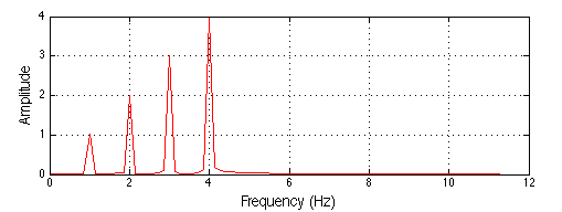
The Spectrum
Intuitively we all know what a spectrum is. For example white light has many colors, each with a different frequency/wavelength. We think of this
distribution of colors as the spectrum of the white light.
We know a lot about frequencies also:
- We change radio stations by changing frequencies
- We change the quality of sounds in players with equalizers which adjust different frequencies
The method of learning the frequency compositionof a signal is known as fourier or spectral analysis.
Fourier/Spectral analysis is used everywhere:
- In spectroscopy/x-ray crystallography to find chemical composition. Watson & Crick used x-ray crystallography to find the sturcutre of DNA.
- In cosmology to find the chemical composition of stars
- In CAT scans and MRIs
- To study mechanical vibrations for the design of aircrafts, bridges, and even concert halls.
- And of course for the analysis, synthesis, and communication of digital signals
Both of these terms (fourier/spectral analysis) have a history behind them so lets digress a little into the history.
Back
History of Spectral Analysis
The idea of a "spectrum" as we known it is less than 300 years old. Analysis techniques are less than 100 years old. Algorithms for analysis are less than 50
years old, but the terminology "spectrum" traces its roots to Newton.
Newton's Discovery
Newton was trying to build a lens for a telscope, but he kept getting rainbow colors instead of white light -- chromatic aberration.
He eventually gave up and invented a parabolic mirror based telescope, but he also continued to study lenses. He theorized that
white light contained all colors and that a prism or lens seperated them. Of course he didn't know why
(Snell's law had not yet been discovered). He managed to prove his theory -- to
the amazement of skeptical colleagues -- by using two prisms, one to disperse the colors:
and another to mix them back to white. He even blocked various component colors to create mixes of subsets of the spectrum at the output of the second prism.
Unfortunately he didn't make the connection to
frequencies - he believed light was corpuscular. He called the colors "ghosts" (specter in Latin) or a spectra.
The spread of colors were the
spectra of white light.
Back
Returning to Frequencies
A note on periodicity:
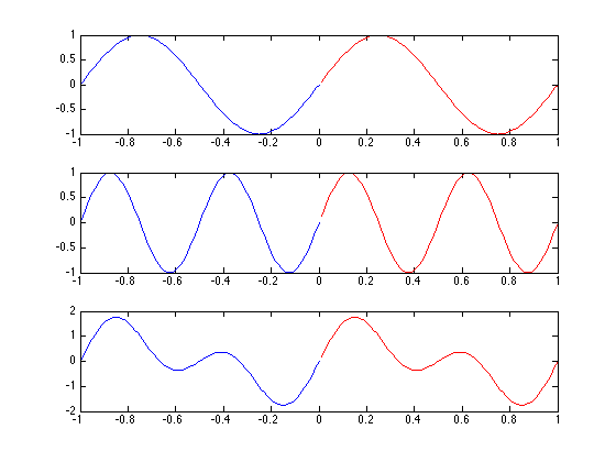
Consider the sum of two sines, one of which is twice the frequency of the other:
\[asin(2 \pi f_o t) + bsin(2 \pi (2f_o) t)\]
The first sine is periodic with time period $T_o = \frac{1}{f_o}$
The second is periodic with period $\frac{T_o}{2} = \frac{1}{2 f_o}$ which is an integral fraction of $T_o$ -- In one cycle of the sinusoid
at $f_o$ we get exactly two cycles of the sinusoid at $2 f_o$
So both of them repeat exactly after a period $T_o$ (this is fundamental period of $sin(2 \pi f_o t)$ & a secondary period of
$sin(2 \pi (2 f_o) t)$. So the SUM of the two also repeats after $T_o$ and it too has a period of $T_o$ -- a fundamental period of $T_o$
Now lets add a their sinusoid at $3f_o$ which has a period $\frac{T_o}{3}$. This too repeats exactly after $T_o$
\[asin(2 \pi f_o t) +bsin(2 \pi (2f_0) t)+csin(2 \pi (3f_o) t)\]
will have a fundamental period of $T_o$
As we keep adding more sinusoids with frequencies that are integer multiples of $f_o$ the sum will remain exactly periodic with $T_o = \frac{1}{f_o}$
In general:
\[s(t) = \sum_{k=0}^{\infty}sin(2 \pi (kf_o)t)\]
will be periodic with time period $T_o=\frac{1}{f_o}$
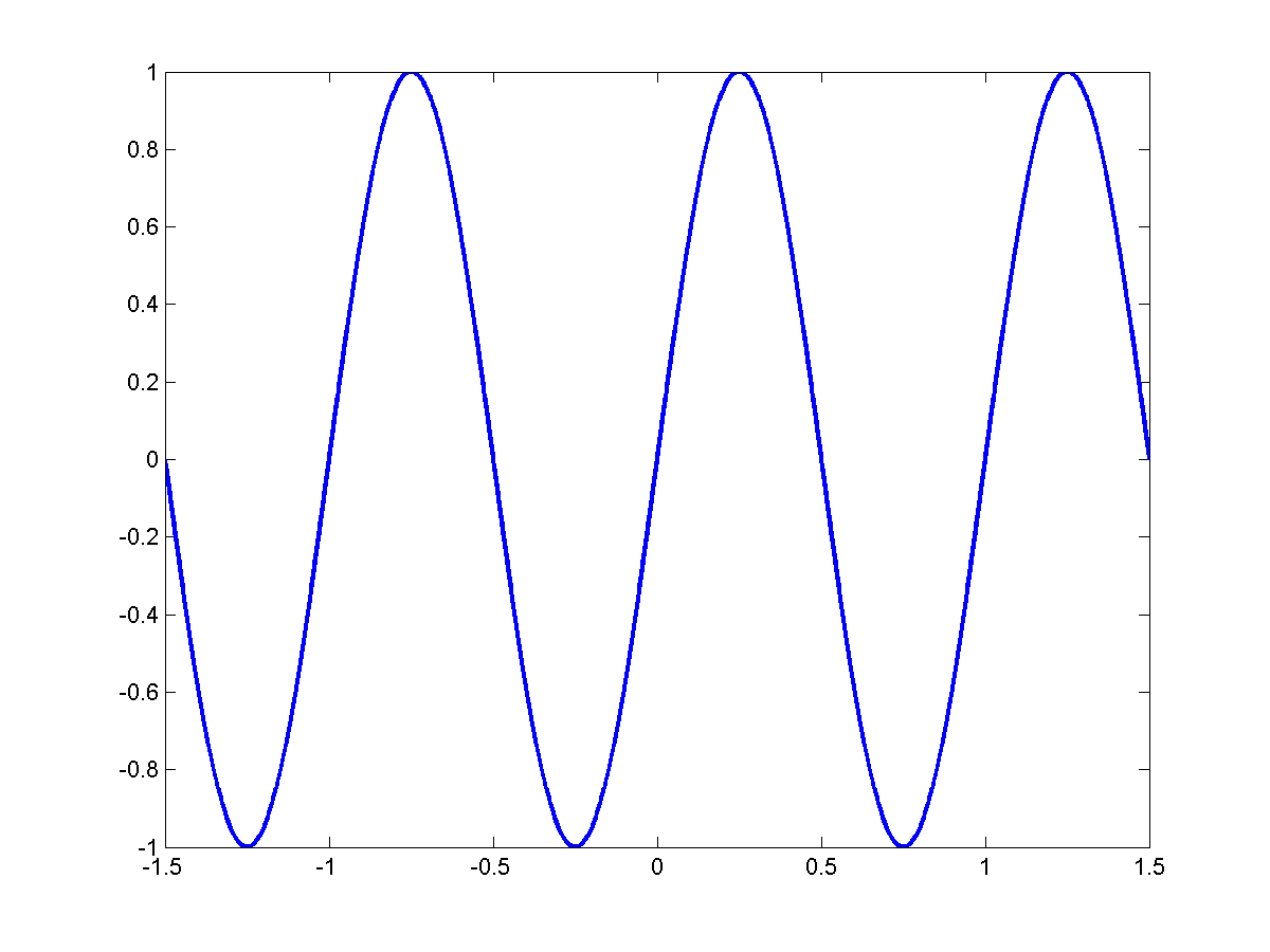
Composing a Sawtooth
Consider
\[sin2 \pi f_o t\]
To this we add:
\[\frac{1}{2}sin2 \pi 2 f_o t\]
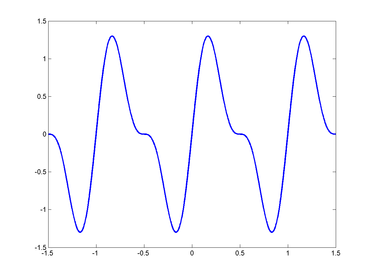
Add:
\[\frac{1}{3}sin(2 \pi 3 f_o) t\]
Each of them is periodic with $T_o = \frac{1}{f_o}$
As we add more and more of these signals together we get this kind of behavior:
 |
$\Rightarrow$ |
 |
$\Rightarrow$ |
 |
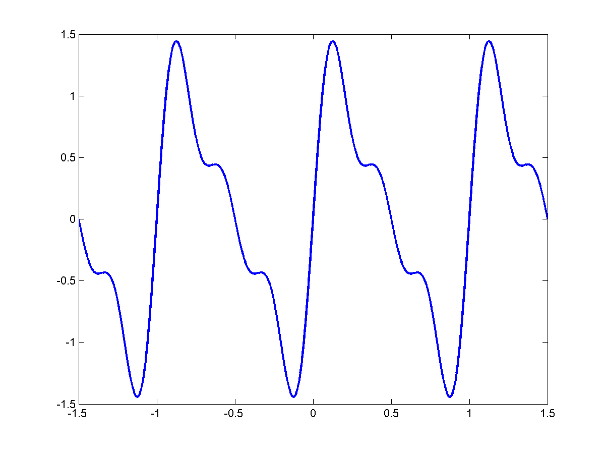
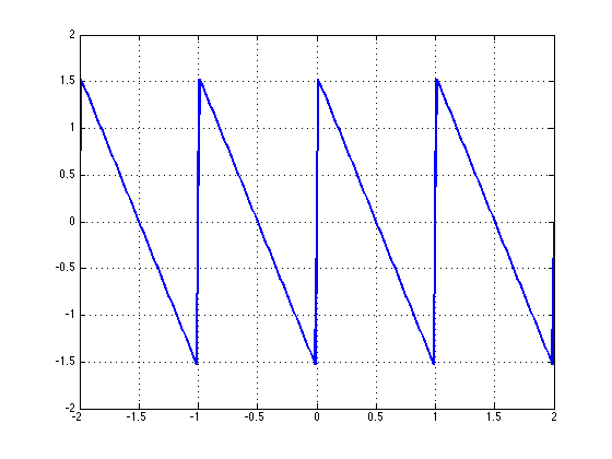
In the limit:
\[\sum_{k=0}^{\infty}\frac{1}{k}sin(2 \pi (kf_o) t)\]
[Insert figure of sawtooth]
We end up with a perfect triangular wave with period $T_o = \frac{1}{f_o}$:
If we consider only the ODD harmonics $f_o, 3f_o, 5f_o, ...$
 |
$f_0$ |
 |
$3f_0$ |
 |
$5f_o$ |
 |
$7f_0$ |
In general:
\[s(t)=\sum_{k=0}^{R}\frac{1}{2k+1}sin(2 \pi (2k+1) f_o t)\]
We get a perfect square wave.
** In fact just about ANY PERIODIC SIGNAL can be expressed as a TRIGONOMETIC SERIES OF HARMONICALLY RELATED SINUSOIDS.**
Back
Returning to History
When the above fact was first realized, it shocked mathmeticians, but then eventually convinced themselves it wasn't true.
Euler was one of the believers. He realized that for a string that is fixed on both ends, the vibrational modes that are permitted require it to be
0 at both ends.
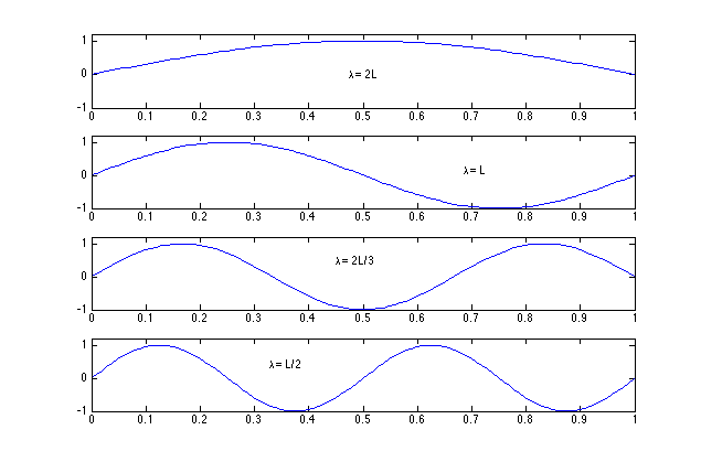
All of these are hornomically related if:
\[f_o = \frac{c}{2L}\]
the modes are $f_o, 2f_o,3f_o, ...$
He also realized that any LINEAR COMBINTTION modes would also be 0 at the ends.
For example one could compose the following:
which is 0 at the ends. Euler proposed that any function that was 0 at the ends could be composed in this way.
But the counter argument was that the following:
[Insert figure of sawtooth w/ points of discontinuity]
has sharp peaks. The sinusoids however are infinitely smooth. We can NEVER construct a signal with sharp discontinuities using smooth signals.
So it was decided that the entire theory - Euler's hypothesis - was wrong so it rested until Joseph Fourier.
Back
Joseph Fourier - a believer - spent a lifetime on this problem. Fourier was a mathmetician who became a famous Eygptologist and then returned
to math to work on this problem. (On the way he also discovered the Greenhouse effect). In summary here are observations he made:
- Considered a sinusoid $sin(2 \pi ft)$ with fundamental period $T = \frac{1}{f}$. It repeats after time T. Any sinusoid whose
frequency is an integer multiple of f also repeats after T although T may not be its fundamental period so:
\[\sum_{n}a_nsin(2 \pi n ft)\]
is also periodic with T as fundamental period
- If we have a signal that is periodic with T it is sufficient to analyze one fundamental period to understand the entire signal. This can be ANY
cycle (starting anywhere).
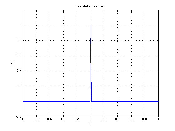
- Let us consider
\[s(t) = \int_{0}^{T}s(\tau)\delta(t - \tau)d \tau , 0 \leq t \leq T\]
according to the above rule. Note that we are only considering $0 \leq t \leq T$ in the integral.
Can we express $\delta(t)$ as a harmonically related trigonometric series? If so, $s(t)$ can also be expressed as a harmonically related trigonometric series.
Let's go back to:
\[\sum_k \frac{sin(2 \pi kft)}{k}\]
What happens if we only add $\sum sin(2 \pi kft)$ or rather (for ease of explanation) $\sum cos(2 \pi kft)$?
\[cos(2 \pi ft)\]
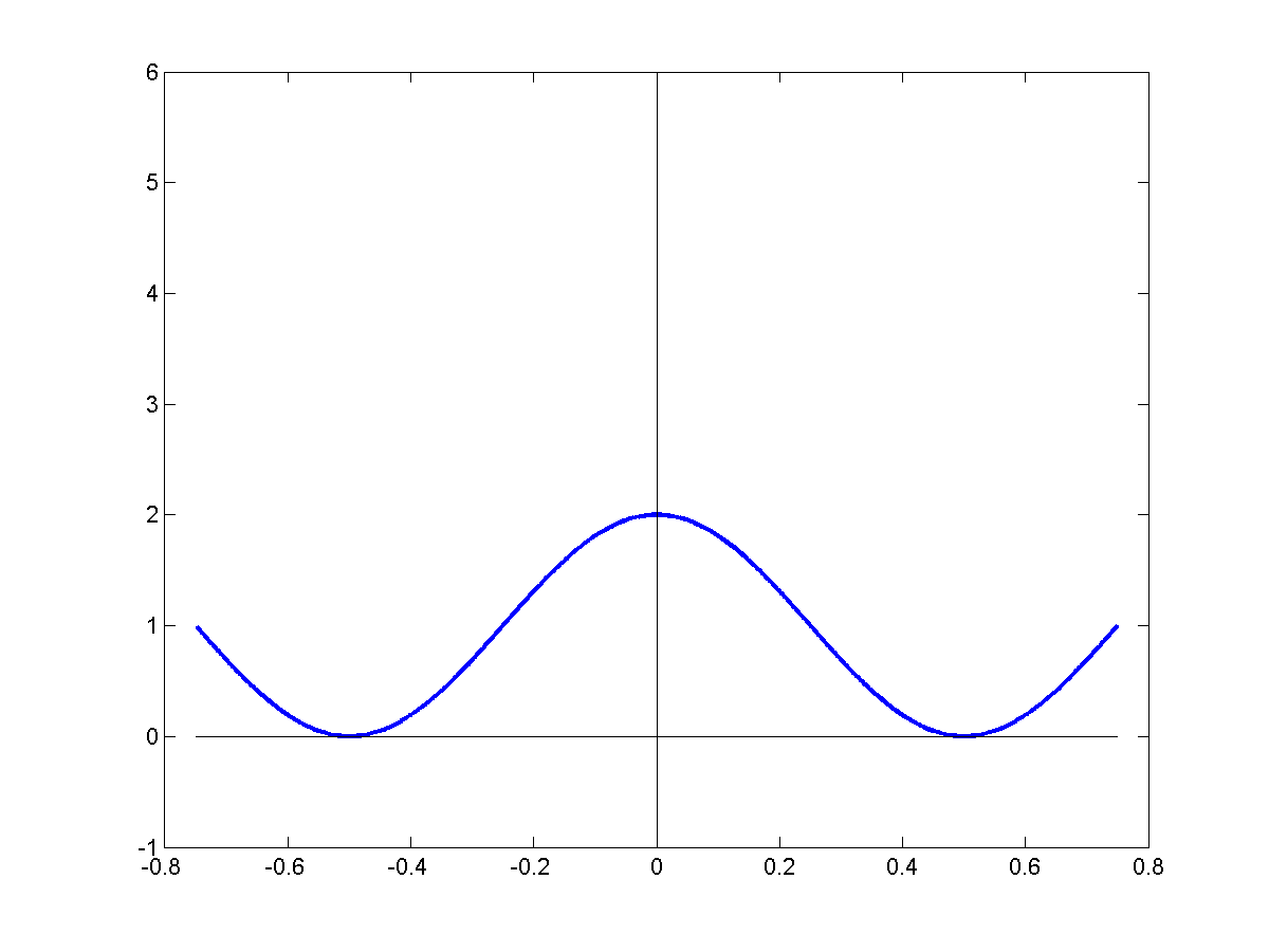
\[cos(2 \pi ft) + cos(2 \pi (2f)t)\]
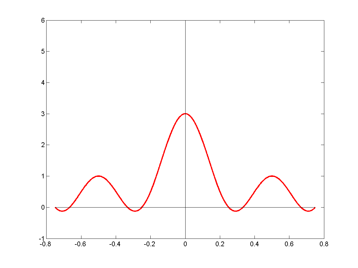
\[cos(2 \pi ft) + cos(2 \pi (2f)t) + cos(2 \pi (3f) t)\]
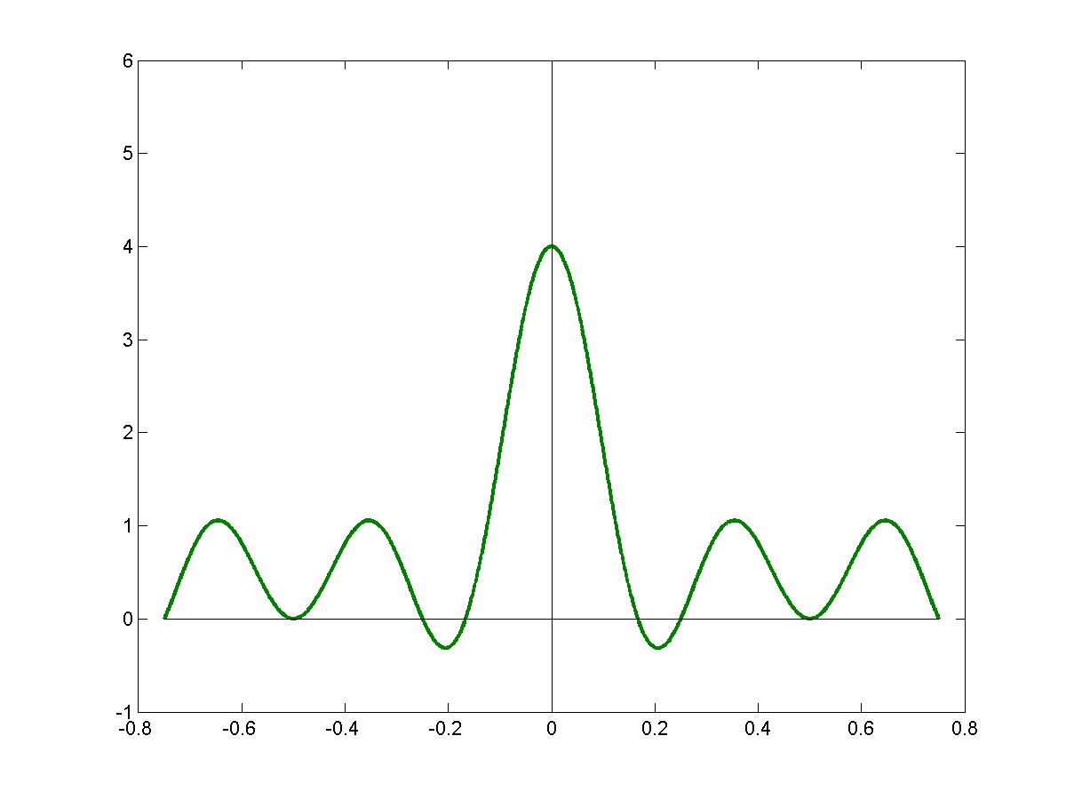
\[\sum_n cos(2 \pi (nf) t)\]
 |
$\Rightarrow$ |
 |
In the limit:
\[\sum_{n=0}^{\infty}cos(2 \pi n ft) = \delta(t)\]
It converges to a delta function.
This is only considering $-\frac{T}{@} \leq t \leq \frac{T}{2}$
This of course repeats with period T. The entire signal will be:
The above series is only centered at t=0. If we want to shift it to $\delta(t-\tau)$ -- i.e. to be centered at "$\tau$"
we must modify the series slighly -- we will shift the cosines.
Note:
\[cos(a+b) = cos(a)cos(b)-sin(a)sin(b)\]
\[cos(2 \pi f(t - \tau)) = cos(2 \pi ft)cos(2 \pi f \tau) - sin(2 \pi f t)sin(2 \pi f \tau)\]
\[\delta(t - \tau) = \sum_{n=0}^{\infty}cos(2 \pi n f \tau)cos(2 \pi n f t) + \sum_{n=1}^{\infty}sin(2 \pi n f \tau)sin(2 \pi n f t)\]
There are two implications to this.
- The first which we will return to later, is that the impulse has a frequency compsition that is also an impulse sequence
- The second gives us the the Fourier Series
\[s(t)=\int_{0}^{T}s(\tau)\delta(t-\tau)d \tau = \sum_{n=0}^{\infty}cos(2 \pi n f t)\int_{0}^{T}s(\tau)cos(2 \pi n f t)d \tau +
\sum_{n=1}^{\infty}sin(2 \pi n f t) \int_{0}^{T}s(\tau)sin(2 \pi n f t)d \tau\]
Back
Fourier Series
Any periodic signal with fundamental period T can be experessed as
\[s(t)=\sum_{n=0}^{\infty}a_n cos(2 \pi n f t) + \sum_{n=1}^{\infty} b_n sin(2 \pi n f t) \text{ where } f = \frac{1}{t} \text{ and}\]
\[a_n=\int_{t_1}^{t_1+T}s(t)cos(2 \pi n f t)dt\]
\[b_n=\int_{t_1}^{t_1+T}s(t)sin(2 \pi n f t)dt\]
Fourier's Theorem
- Any periodic (CT) signal can be expressed as the sum of harmonically related sines & consines as
\[s(t)=\sum_{n=0}^{\infty}a_ncos(2 \pi n f t) + \sum_{n=1}^{\infty}b_nsin(2 \pi n f t)\]
- This representation is unique
We have shown (1). Can we prove uniqueness?
We start with the following observation:
\[\int_{0}^{T}sin\frac{2 \pi n_1 t}{T} sin \frac{2 \pi n_2 t}{T} =
\begin{cases}
0, & n_1 \neq n_2 \\
\frac{T}{2}, & n_1 = n_2
\end{cases}
\]
Proof
First consider $n_1 = n_2$:
\[F = \int_{0}^{T}sin^2(\frac{2 \pi n_1 t}{T})dt\]
Since the signal $sin^2(2 \pi n_1 t)$ is periodic it does not matter which period we integrate over. Shifting forward by half a cycle gives us the same result:
\[F = \int_{0}^{T}sin^2(\frac{2 \pi n_1 t}{T})dt = \int_{0}^{T}cos^2(\frac{2 \pi n_1 t}{T})dt\]
\[
\begin{align*}
2F &= \int_{0}^{T} \left(sin^2(\frac{2 \pi n_1 t}{T})dt + cos^2(\frac{2 \pi n_1 t}{T}) \right )dt\\
&= \int_{0}^{T}1dt = T \Rightarrow F = \frac{T}{2}
\end{align*}
\]
Now consider $n_1 \neq n_2$. Pictorically consider
\[sin(\frac{2 \pi n_1 t}{T})\]
The positive regions ancel out the negative regions for:
\[sin(\frac{2 \pi n_2 t}{T})\]
Now consider:
\[sin(\frac{2 \pi n_1 t}{T}) * sin(\frac{2 \pi n_2 t}{T})\]
The positive and negative regions will canel out! So the total area is 0. We can prove it trigonomentrically using the smae logic as before:
\[f = \int_{0}^{T}sin(\frac{2 \pi n_1 t}{T})sin(\frac{2 \pi n_2 t}{T})dt\]
Recall:
\[sinasinb=\frac{1}{2}(cos(\frac{a-b}{2})-cos(\frac{a+b}{2}))\]
\[\text{So } f = \frac{1}{2}\int_{0}^{T}cos\frac{2 \pi (n_1-n_2)}{2T}dt - \frac{1}{2}\int_{0}^{T}cos\frac{2 \pi (n_1+n_2)}{2T}dt\]
\[\text{For } n_1 \neq n_2 \text{ f = 0}\]
To prove uniqueness let us assume there are two different harmonic series representations for $s(t)$:
\[s(t) = \sum_{n=0}^{\infty}a^1_n cos2 \pi n f t + \sum_{n=1}^{\infty}b^1_n sin 2 \pi n f t\]
\[s(t) = \sum_{n=0}^{\infty}a^2_n cos2 \pi n f t + \sum_{n=1}^{\infty}b^2_n sin 2 \pi n f t\]
Multiply both representatins by $sin(2 \pi n_1 f t)$ and integrate over $[0,T)$
\[\Rightarrow \sum_{n=0}^{\infty}a^1_n \int_{0}^{T} cos(2 \pi n f t) sin (2 \pi n_1 f t) dt + \sum_{n=1}^{\infty}b^1_n \int_{0}^{T} sin(2 \pi n f t)sin (2 \pi n_1 f t) dt\]
\[s(t) = \sum_{n=0}^{\infty}a^2_n \int_{0}^{T} cos(2 \pi n f t)sin (2 \pi n_1 f t) dt + \sum_{n=1}^{\infty}b^2_n \int_{0}^{T}sin(2 \pi n f t)sin (2 \pi n_1 f t) dt\]
\[\text{Since } \int_{0}^{T} cos(2 \pi n f t)sin (2 \pi m f t) dt = 0 \forall n \neq m\]
\[\text{And } \int_{0}^{T} sin(2 \pi n f t)sin (2 \pi m f t) dt = 0 \forall n \neq m \]
We set:
\[b_n^2 \int_{0}^{T}sin(2 \pi n f t)sin(2 \pi n_1 f t)dt = b_n^2 \int_{0}^{T}sin(2 \pi n_1 f t)sin(2 \pi n f t)dt\]
\[\Longrightarrow b_{n}^1 \frac{T}{2} = b_{n}^2 \frac{T}{2}\]
\[\Longrightarrow b_{n_1}^1 = b_{n_1}^2\]
The "b" terms are identical for both expansions. We can similarily show the "a" terms are identical in both expansions. I.e. the two
expansions are identical. Therefore the series representation is uniqe.
Let us now offically derive $a_n$ & $b_n$ ($f = \frac{1}{T}$)
\[s(t) = \sum_{n=0}^{\infty}a_ncos(2 \pi n f t) + \sum_{n=1}{\infty}b_n sin(2 \pi n f t)\]
Multiplying both sides by $sin(2 \pi m ft)$ and integrating over $[0,T)$ and using out rules about the integral terms that go to 0.
\[
\begin{align*}
\int_{0}^{T}s(t)sin(2 \pi m f t)dt &= \sum_{n=0}^{\infty}a_n \int_{0}^{T}cos(2 \pi n f t)sin(2 \pi m f t) + \sum_{n=1}^{\infty}b_n \int_{0}^{T}sin(2 \pi n f t)sin(2 \pi m f t) \\
&= 0 + b_m \frac{T}{2}
\end{align*}
\]
\[b_m = \frac{2}{T} \int_{0}^{T}s(t)sin(2 \pi m f t)dt\]
Similarly multiplying by $cos(2 \pi m f t)$ & integrating over $[0,T)$ we will get
\[a_m = \frac{2}{T} \int_{0}^{T}s(t)cos(2 \pi m f t)dt\]
Special case $m = 0$, simply integrate $s(t)$ wihtout multiplying anything:
\[
\begin{align*}
\int_{0}^{T}s(t)dt &= a_o \int_{0}^{T}dt + \sum_{n=1}^{\infty}a_n \int_{0}^{T}cos(2 \pi n f t)dt + \sum_{n=1}^{\infty}b_n sin(2 \pi n f t)dt \\
&= a_oT + 0 + 0
\end{align*}
\]
\[a_o = \frac{1}{T} \int_{0}^{T}s(t)dt\]
Back
Fourier Series Expansion
Any periodic signal with fundamental period T can be written as:
\[s(t) = \sum_{n=0}^{\infty}a_n cos(2 \pi n f t) + \sum_{n=1}^{\infty}b_n cos(2 \pi n f t), 0 \leq t \leq T\]
\[\text{Where } a_o = \frac{1}{T} \int_{0}^{T}s(t)dt\]
\[a_n = \frac{2}{T} \int_{0}^{T}s(t)cos(2 \pi n f t)dt, n > 0\]
\[b_n = \frac{2}{T} \int_{0}^{T}s(t)sin(2 \pi n ft)dt\]
where $f = \frac{1}{T}$ is the fundamental frequency of the signals.
The above process we also learned that $\sqrt{\frac{2}{T}}sin(2 \pi n f t)$ and $\sqrt{\frac{2}{T}}cos(2 \pi n f t)$
are orthogonal bases. We are expressing $s(t)$ as a weighted combination of orthogonal bases. The simplicity of the derivation dervies from the orthogonality.
Some Examples
-
$s(t) = Asin2 \pi f t + B$
\[
\begin{align*}
a_o &= \frac{1}{T} \int_{0}^{T}s(t)dt = \frac{1}{T} \int_{0}^{T}A sin (2 \pi f t)dt + \frac{1}{T} \int_{0}^{T} Bdt \\
&= B
\end{align*}
\]
\[
\begin{align*}
a_n &= \frac{2}{T} \int_{0}^{B} Asin (2 \pi ft) cos (2 \pi n f t) dt + \frac{2}{T} \int_{0}^{T} B cos (2 \pi n ft)dt\\
&= 0, n > 0
\end{align*}
\]
\[
\begin{align*}
b_n &= \frac{2}{T} \int_{0}^{T} Asin(2 \pi ft) sin(2 \pi nft)dt + \frac{2}{T \int_{0}^{T}} Bsin (2 \pi ft)dt \\
&= \begin{cases}
A , & n = 1 \\
0, & n \neq
\end{cases}A
\end{align*}
\]
-
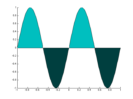
Lets derive the Fourier Series expansion for the following version of the square wave:
\[
s(t) = \begin{cases}
1, & 0 \leq t < \frac{T}{2} \\
-1, -\frac{T}{2} \leq t < T \\
s(t + T) \text{ in general}
\end{cases}
\]
\[
\begin{align*}
a_o &= \frac{1}{T} \int_{0}^{T}s(t)dt \\
&= \frac{1}{T} \int_{0}^{\frac{T}{2}}dt - \int_{\frac{T}{2}}^{T}dt \\
&= \frac{1}{T} (\frac{T}{2} - \frac{T}{2}) \\
&= 0
\end{align*}
a_o = 0
\]
\[
a_n = \frac{2}{T} \left( \int_{0}^{\frac{T}{2}} cos \frac{2 \pi nt}{T}dt - \int_{\frac{T}{2}}^{T}cos \frac{2 \pi n t}{t}dt \right) , n > 0
\]
\[\text{Let } t' = T - t \rightarrow dt = -dt'\]
\[t = T - t'\]
\[
\begin{align*}
cos \frac{2 \pi n t}{T} &=cos \frac{2 \pi n (T - t')}{T} \\
&= cos \frac{2 \pi n T}{T} cos \frac{2 \pi n t'}{T} - sin\frac{2 \pi n T}{T} sin \frac{2 \pi n t'}{T}
\end{align*}
\]
\[\text{From: } cos(a-b) = cosacosb + sinasinb\]
\[cos \frac{2 \pi n T}{T} = cos 2 \pi n = 1\]
\[sin \frac{2 \pi n T}{T} = sin 2 \pi = 0\]
\[cos \frac{2 \pi n}{T}(T - t') = cos \frac{2 \pi n t'}{T}\]
\[
\begin{align*}
a_n &= \frac{2}{T} \left[ \int_{0}^{\frac{T}{2}} cos \frac{2 \pi n t}{T}dt - \int{\frac{T}{2}}^{T}cos \frac{2 \pi nt}{T}dt \right] \\
&= \frac{2}{T} \left[ \int_{0}^{\frac{T}{2}} cos \frac{2 \pi n t}{T}dt - \int{\frac{T}{2}}^{0}cos \frac{2 \pi nt'}{T}(-dt') \right] \\
&= \frac{2}{T} \left[ \int_{0}^{\frac{T}{2}} cos \frac{2 \pi n t}{T}dt - \int{0}^{\frac{T}{2}}cos \frac{2 \pi nt'}{T}(-dt') \right] \\
&= 0, n >0
\end{align*}
\]
You can understand this pictorially by drawing:
\[s(t)cos \frac{2 \pi n t}{T}\]
For $n = 1$ these areas are identical, but have opposite sign & cancel out.
For $n = 2$
\[
\begin{align*}
b_n &= \frac{2}{T} \int_{0}^{T}s(t)sin \frac{2 \pi n t}{T} \\
&=\frac{2}{T}\left[ \int_{0}{\frac{T}{2}} sin \frac{2 \pi nt}{T}dt - \int_{\frac{T}{2}}^{T}sin \frac{2 \pi n t}{t}dt\right]
\end{align*}
\]
\[\text{Let } t' = T - t \rightarrow dt = -dt'\]
\[t = T - t'\]
\[
\begin{align*}
sin \frac{2 \pi n t}{T} &= \\
&=sin \frac{2 \pi n (T - t')}{T} \\
&= sin \frac{2 \pi n T}{T} cos \frac{2 \pi n t'}{T} - cos\frac{2 \pi n T}{T} sin \frac{2 \pi n t'}{T}
\end{align*}
\]
\[\text{From: } sin(a-b) = sinacosb - cosasinb\]
\[sin \frac{2 \pi n T}{T} = sin 2 \pi n = 0\]
\[cos \frac{2 \pi n T}{T} = cos 2 \pi = 1\]
\[\Rightarrow sin \frac{2 \pi n}{T}(T - t') = cos \frac{2 \pi n t'}{T}\]
\[
\begin{align*}
b_n &= \frac{2}{T} \left[ \int_{0}^{\frac{T}{2}} sin \frac{2 \pi n t}{T}dt - \int{\frac{T}{2}}^{T}-sin \frac{2 \pi nt}{T}(-dt) \right] \\
&= \frac{2}{T} \left[ \int_{0}^{\frac{T}{2}} sin \frac{2 \pi n t}{T}dt - \int{\frac{T}{2}}^{0}sin \frac{2 \pi nt'}{T}dt' \right] \\
&= \frac{2}{T} \left[ \int_{0}^{\frac{T}{2}} sin \frac{2 \pi n t}{T}dt + \int{0}^{\frac{T}{2}}sin\frac{2 \pi nt'}{T}dt \right] \\
&= \frac{4}{T} \int_{0}^{\frac{T}{2}}sin \frac{2 \pi n t}{T}dt, n >0
\end{align*}
\]
Try plotting $sin \frac{2 \pi n t}{T}$ of $(0, \frac{T}{2})$
When n is even, you get $\frac{n}{2}$ cycles in $\frac{T}{2}$
There are $\frac{n}{2}2$ FULL cycles in $\frac{T}{2}$. In each cycles the positive part of the cycle cancels out the negative
part of the cycles. Therefore the net area is 0. Hence:
\[b_n = 0 \text{ for even n}\]
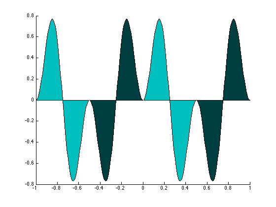
What happens when n is odd?
We get $\frac{n}{2}$ cycles of $\frac{T}{2}$. Of these, for all but the final half cycle, the positive and negative areas cancel out.
We only get the net area of one half cycle!
\[\int_{0}^{\frac{T}{2}}sin \frac{2 \pi n t}{T}dt = \int_{0}^{\frac{T}{2n}}sin2 \pi (\frac{n}{T})tdt = \frac{T}{\pi n}\]
\[b_n = \frac{4}{\pi n} \text{ for n = odd } \]
\[\text{**Note: } \int_{0}^{\pi}sinxdx =2\]
The Fourier Series of:
\[
s(t) = \begin{cases}
1, & 0 \leq t < \frac{T}{2} \\
-1, -\frac{T}{2} \leq t < T \\
s(t + T) \text{ in general}
\end{cases}
\]
is
\[a_n = 0,\]
\[b_n = 0 \text{ for even } n\]
\[b_n = \frac{4}{\pi n} \text{ for odd } n\]
Back
Returning to Euler/Lagrange's Problem with Discontinuities - Gibbs Phenomenon
Michaelson's Discovery
Albert Michaelson won the first nobel for proving that the speed of light is constant. Not well known is that as part
of his work he built the first Fourier analysis device. He used it to show Fourier was right. But he recieved some weird results.
For square waves, the fourier series did not coverge well. As he adds more and more terms the series approximation ALWAYS had some ringing.
He thought he may have had a bug in his machine so he went to Josiah Gibbs with his problem. Gibbs refered to old work by Dirchlet
and realized Michaelson's problem was due to discontinuites in the square wave. The Fourier series misbehaved if there were discontinuties
in the signal. This phenomenon now called the Gibbs phenomenon was published in Natuure in 1889.
Dirchlet's Condition
Dirchlet was Fourier's student and proved the following, For a periodic signal $s(t)$, the Fourier Series always converges if and only if:
- $s(t)$ is absolutely integrable
\[\int_{0}^{T}|s(t)|dt < \infty\]
-
$s(t)$ uas an infinite number of extrema over a period.
- $s(t)$ has a finite number of discontinuities in any period
But what do we mean by "converge"? Let us represent the series expansion generally as:
\[s(t)=s_0(t)+s_1(t) +s_2(t)+ \dots\]
where $s_n(t)$ has sine and cosine terms with frequency $nf$
\[\int_{0}^{T}|s(t)-s_0(t)|^2dt \geq \int_{0}^{T}|s(t) - (s_0(t)+s_1(t))|^2dt \geq \int_{0}^{T}|s(t) - (s_0(t)+s_1(t) + s_2(t))|^2dt\]
Or more general:
\[\text{For } N < \mu, \int_{0}^{T}|s(t)-\sum_{i=0}^{N}s_i(t)|^2dt \geq \int_{0}^{T}|s(t) - \sum_{i=0}^{\mu}s_i(t)|^2dt\]
As we increase the number of terms the $L_2$ error between $s(t)$ and series approximation decreases.
But this does not mean that the actualy error goes to 0, only that the area under the squared error function got to 0.
You can still have very high error at one point for instance if the width over which you have the error is so small that the area of the error is 0.
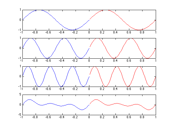
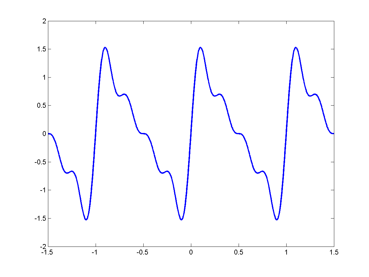
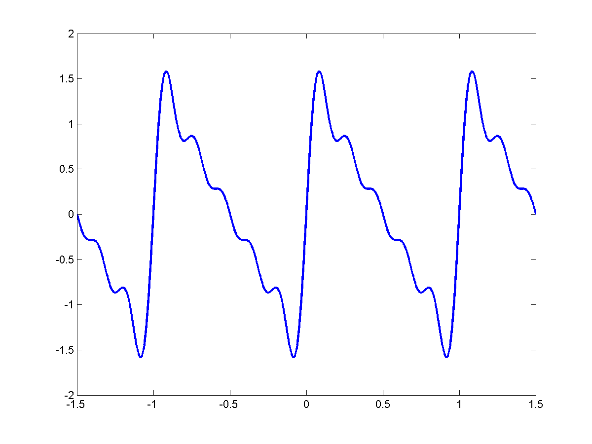
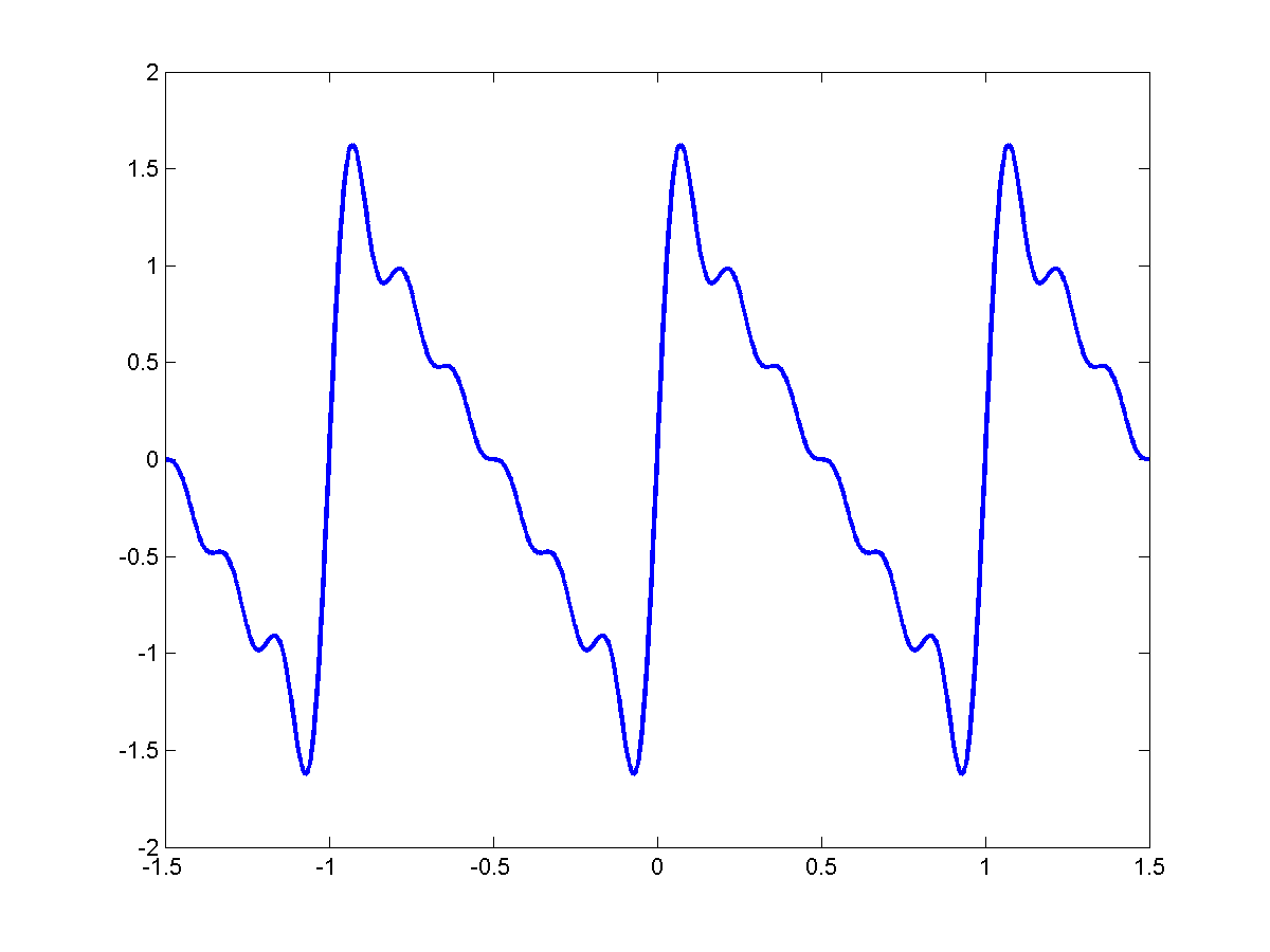
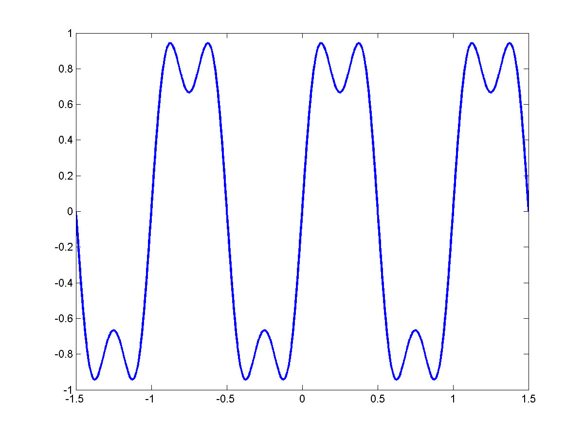
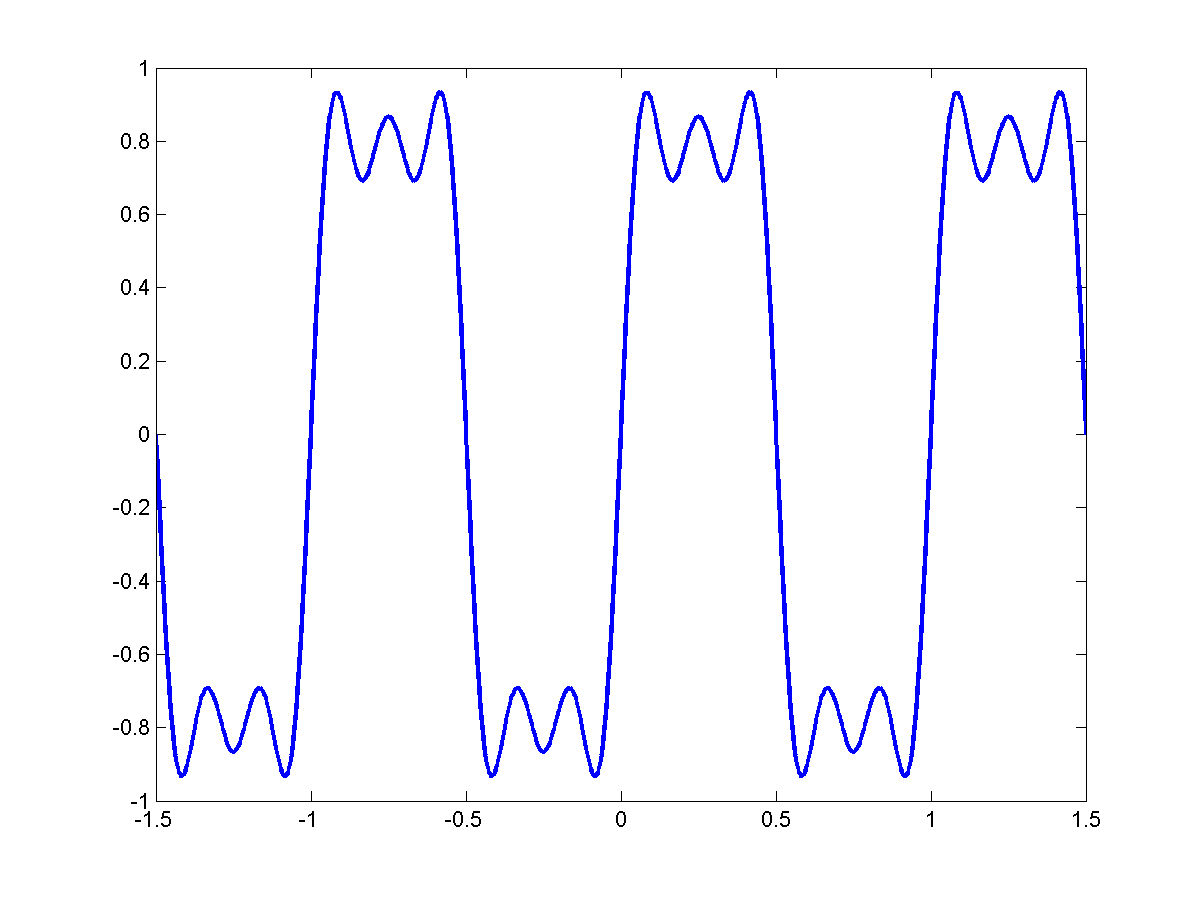
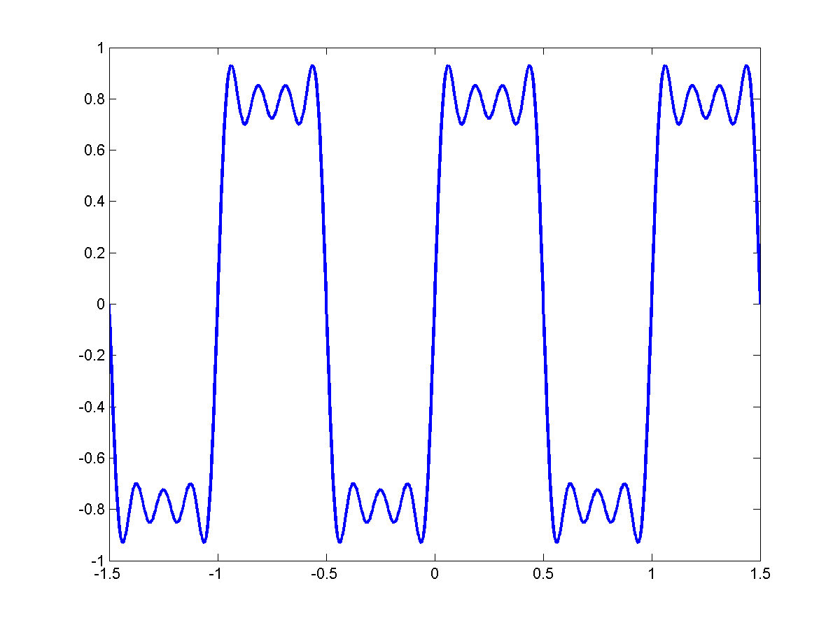
Consider the squares wave. The figure below show:
\[s(t), s_1(t), s_1(t)+s_2(t), s_1(t)+s_2(t)+s_3(t)\]
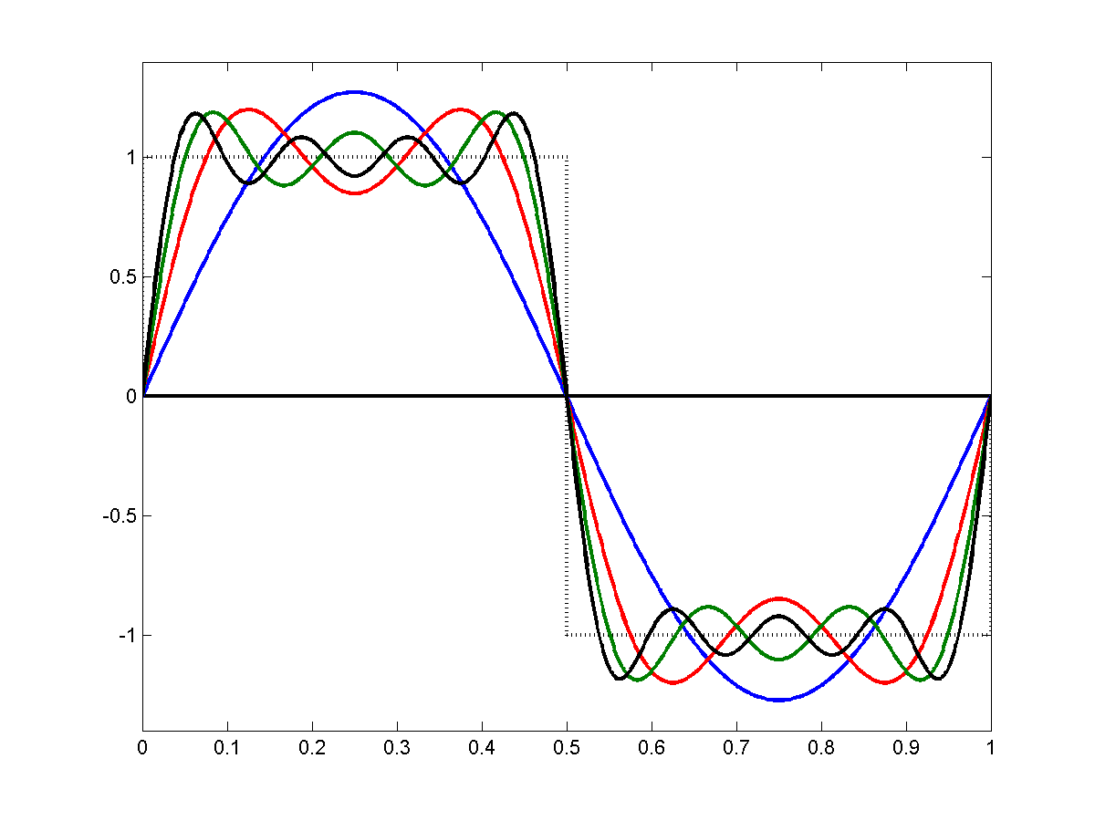
As you keep adding more terms, the series gets closer to the square wave but the "ringing" never really goes away. You will
always have an overshoot at the discontinuities.
More Dirichlet's Theorem: At discontinuties the series converges to the mid-point. To understand this, let's take the following example.
Consider:
\[
\begin{align*}
D_x(t) &= \frac{1}{2} + cos(t) + cos(2t) + cos(3t) + \dots + cos(kt) \\
&= \frac{1}{2} + \sum_{n=1}^{K}cos(nt) \\
&= \frac{sin((k+\frac{1}{2})t)}{2sin(\frac{t}{2})}
\end{align*}
\]
Using this results and little trigonometry we can show that for any periodic signal $s(t)$ with period T, the Fourier Series for $s(t)$ is:
\[s(t) = \sum_{n=0}^{\infty}a_ncos \frac{2 \pi n t}{T} + \sum_{n=1}^{\infty}b_nsin \frac{2 \pi n t}{T}\]
\[s_K(t) = \sum_{n=0}^{K}a_ncos \frac{2 \pi n t}{T} + \sum_{n=1}{K} b_n sin \frac{2 \pi nt}{T}\]
\[s_K(t) = \frac{2}{T} \int_{0}^{T} s(t+\tau)D_K(\frac{2 \pi}{T} \tau) d \tau\]
We now introduce two improtant functions:
\[sinc(t) = \frac{sint}{t}\]
\[Sinc(t) = \int_{0}^{T} sinc(t)dt\]
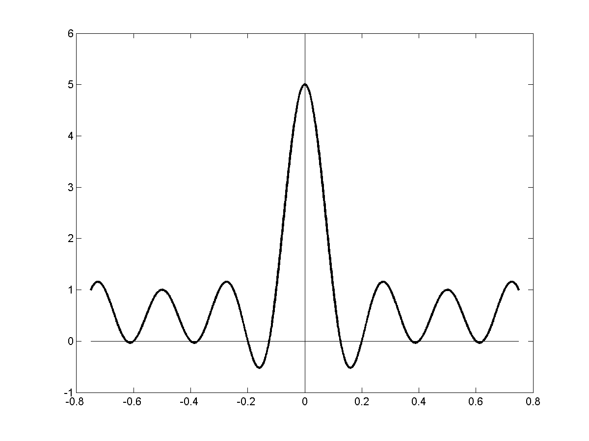
Sinc(t) looks like this
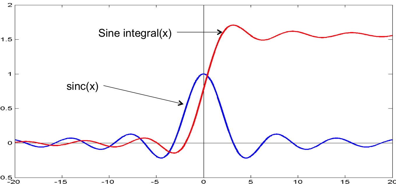
Close to $t=0$, the $k^{th}$ order series approximation of the square wave approximates.
\[s_K(t) = \frac{2}{\pi}sgn(t) Sinc(4 \pi k |t|)\]
The max value of Sinc(x) occurs at $x = \pi$
The max value of $s_K(t)% will occur at $4 \pi kt = \pi \Rightarrow t = \frac{1}{4k}$
As the order of the series increases the peak error in approximation will approach 0. But the peak error is not going to go
below 9%
Another characteristic of the Sinc is that its amplitude decays as $\frac{1}{t}$
So for every doubling of the distance from the discontinuity the overshoot is halved. For very large K, the first peak
occrs at $\frac{1}{k}$ and the oscillation subsides to 0 very quickly.
What is the implication?
A discontinuity represents an infinite frequency event. When you use K terms to approximate it you are approximating it with a bandwidth of K*f.
This means that withing $\frac{1}{Kf}$ ($=\frac{T}{k}$) of the discontinuity the approximation will not approach the true signal. We do have
through $-\infty$ then coefficient decrease rapidly with increasing $n$.
This is true not just for square waves but for any discontinuties signal including triangle sawtooth etc.
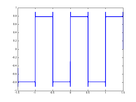
Gibb's Phenomenon
Whenever a signal has jump discontinuties the F.S. converges at jump time to the midpoint of the jump.
Partial sums oscillate before & after the jump. The number of cycles of oscillation is equal to the number of terms in the series.
The size of the overshoot decrease with the number of terms approaching 9% of the jump.
Note on Phase
So far we have considered F.S. of the form:
\[s(t) = a_0 + a_1cos 2 ]pi ft + a_2 cos 2 \pi (2f)t + \dots + b_1sin2 \pi ft + b_2 sin 2 \pi (2f)t + \dots\]
This includes both sines and cosine components.
In reality you don't need both. You can have series entirely in terms of sines, or entirely in cosines if you include a phase.
For example we can say:
\[s(t) = a_0 + \sum_{k=1}^{\infty}a_kcos(\frac{2 \pi k t}{T + \phi_k})\]
\[\text{OR}\]
\[s(t) = b_0 + \sum_{k=1}^{\infty}sin(\frac{2 \pi kt}{T} + \phi_k)\]
This is more intuitive since it explicitly shows the contribution of a frequency. However the problem is that we will now have
to estimate the phase $\phi_k$ which is not simple.
Back
Fourier Series with Complex Exponentials
Another way to avoid having both sines & consine is the express them as complex exponentials:
\[sin(\theta) = \frac{1}{2j} (e^{j \theta} - e^{-j \theta}) = \frac{-j}{2}(e^{j \theta} - e^{-j \theta})\]
\[cos(\theta) = \frac{1}{2}(e^{j \theta} + e^{-j \theta}) \]
\[
\begin{align*}
b_ksin \frac{2 \pi k t}{T} + a_k cos \frac{2 \pi k t}{T} =&\\
&= (\frac{a_k}{2} - \frac{jb_k}{2})e^{j \frac{2 \pi k t}{T}} + (\frac{a_k}{2} + \frac{jb_k}{2})e^{-j \frac{2 \pi k t}{T}}
\end{align*}
\]
\[
\begin{align*}
\text{Letting } r_k &= \frac{a_k}{2} - \frac{jb_k}{2} \\
&= r_k e^{\frac{j2 \pi kt}{T}} + r_k e^{\frac{-j 2 \pi k t}{T}}
\end{align*}
\]
$r_k$ tells us all we need to know. This tells us we can simply express F.S. in terms of complex exponentials
\[s(t) = \sum_{k = -\infty}^{\infty} C_k e ^{\frac{2 \pi k t}{T}}\]
This is a simplier form of series expansion but comes at a cost. We now have to consider negative frequencies.
How to Derive $C_k$
Note:
\[
\int_{0}^{T}e^{\frac{j2 \pi kt}{T}}e^{\frac{-j2 \pi lt}{T}} =
\begin{cases}
T, & k = l \\
0, otherwise
\end{cases}
\]
For example complex exponentials are orthogonal:
\[ \int_{0}^{T}s_1(t)s_2^*(t) = 0\]
So
\[s(t) = \sum_{k = -\infty}^{\infty}C_k e ^{\frac{j2 \pi kt}{T}}\]
\[
\begin{align*}
\int_{0}^{T}s(t)e^{\frac{-j2 \pi lt}{T}}dt &= \sum_{k = -\infty}^{\infty}C_k e^{\frac{j2 \pi kt}{T}} e^{\frac{-j2 \pi kt}{T}}dt \\
&= T * C_l
\end{align*}
\]
\[C_l = \frac{1}{T} \int_{0}^{T}s(t) e^{\frac{-j2 \pi l t}{T}}dt \]
We will hence forth only use the complex exponential F.S.:
\[s(t) = \sum_{k = -\infty}^{\infty} C_k e^{\frac{j2 \pi kt}{T}}\]
\[C_k = \frac{1}{T} \int_{0}^{T}s(t) e^{\frac{-j2 \pi kt}{T}}dt\]
What is negative frequency (i.e -100Hz)? Think of a phasor in a complex plane. Positive frequencies represent a phasor that is rotating
counter clockwise. Negative freqencies represent a phasor that is rotating clockwise.
EXAMPLE
-
$s(t) = Acos \frac{2 \pi}{T}t$
\[
\begin{align*}
C_k &= \frac{1}{T} \int_{0}^{T}A cos \frac{2 \pi}{T}t e^{\frac{-j 2 \pi k}{\tau}t}dt \\
&= \frac{A}{2T} \left[ \int_{0}^{T} e^{\frac{j2 \pi t}{T}} e^{\frac{-j2 \pi kt}{T}}dt + \int_{0}^{T}e^{\frac{-j2 \pi t}{T}} e^{\frac{-j2 \pi kt}{T}}dt\right]
&= \frac{A}{2T} \delta(k-1) + \frac{A}{2T} \delta(k+1)
\end{align*}
\]
Note the frequency axis is discrete.
Relating comples expontenial to quadrature FS
\[a_k = C_k + C_{-k}\]
\[b_k = j(C_k - C_{-k})\]
Properties of the Fourier Series
- Linearity
\[\text{If } s_1(t) \rightarrow C_k\]
\[s_2(t) \rightarrow d_k\]
\[\text{Then } s_1(t) + b s_2(t) \rightarrow a C_k + bd_k\]
-
Time-shift
\[s(t) \rightarrow C_k\]
\[s(t - \tau) \rightarrow C_k e^{\frac{-j2 \pi k \tau}{T}}\]
-
Parseval's Theorem
\[\frac{1}{T} \int_{0}^{T}|s(t)|^2dt = \sum_{k = -\infty}^{\infty}|C_k|^2\]
Easily proved by wriing s(t) as a series & squaring it on the LHS.
-
For real signals:
\[s(t) = s^*(t)\]
\[C_k = C_{-k}^*\]
\[
\begin{align*}
C_{-k} = \int_{0}^{T}s(t)e^{\frac{j 2 \pi kt}{T}}dt
C_{-k}^* = \int_{0}^{T}s(t)e^{\frac{-j2 \pi kt}{T}}dt
\end{align*}
\]
See complete list of properties here
Back
The Fourier Series of a Pulse Train
Let's consider a Fourier series of a pulse Train of duty cycle
\[\frac{d}{T}=D\]
\[s(t) =
\begin{cases}
1, & 0 \leq |t| < \frac{d}{2} \\
0, & \frac{d}{2}\leq |t| < \frac{T}{2} \\
s(t+T), & otherwise
\end{cases}
\]
\[
\begin{align*}
C_k &= \frac{1}{T} \int_{\frac{-T}{2}}^{\frac{T}{2}}s(t)e^{\frac{-j2 \pi kt}{T}}dt \\
&= \frac{1}{T} \int_{\frac{-d}{2}}^{\frac{d}{2}}e^{\frac{-j 2 \pi kt}{T}}dt \\
&= \frac{1}{T}*\frac{T}{-2j \pi k} \bigg|_{-\frac{d}{2}}^{\frac{d}{2}}e^{\frac{-j2 \pi k t}{T}} \\
&= \frac{-1}{j 2 \pi k}\left( e^{\frac{-j 2 \pi k}{T} \frac{2}{2}}-e^{\frac{j 2 \pi k}{T} \frac{d}{2}}\right) \\
&= \frac{1}{\pi k} \left( \frac{e^{\frac{j \pi k d}{T}} - e^{\frac{-j \pi k d}{T}}}{2j}\right) \\
&= \frac{sin \frac{\pi k d}{T}}{\pi k} \\
&= \frac{d}{T} \frac{sin \frac{\pi k d}{T}}{\pi k \frac{d}{T}}
\end{align*}
\]
$\frac{d}{T} = D$ Which is the duty cycle so:
\[C_k = Dsin \pi k D\]
THE FOURIER SERIES DEPENDS ONLY ON THE DUTY CYCLE D & NOT ON THE TIME PERIOD T. BUT THE ACTIVE FREQUENCIES (in $e^{\frac{j2 \pi kt}{T}}$)
DEPEND ON "T"
\[C_k = Dsin \pi k D\]
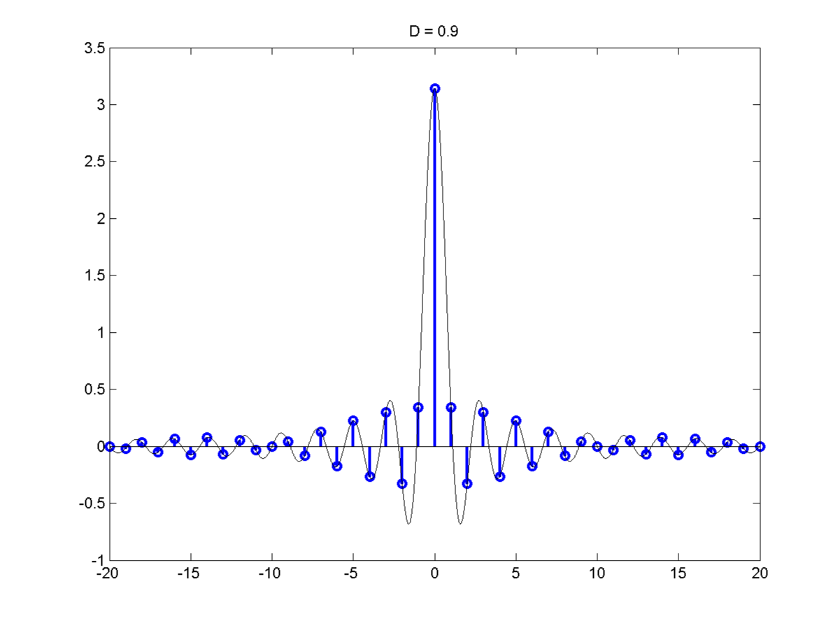
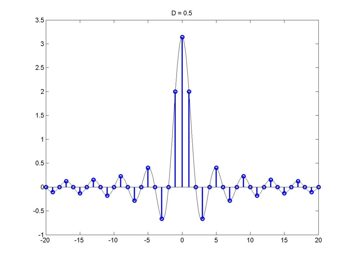
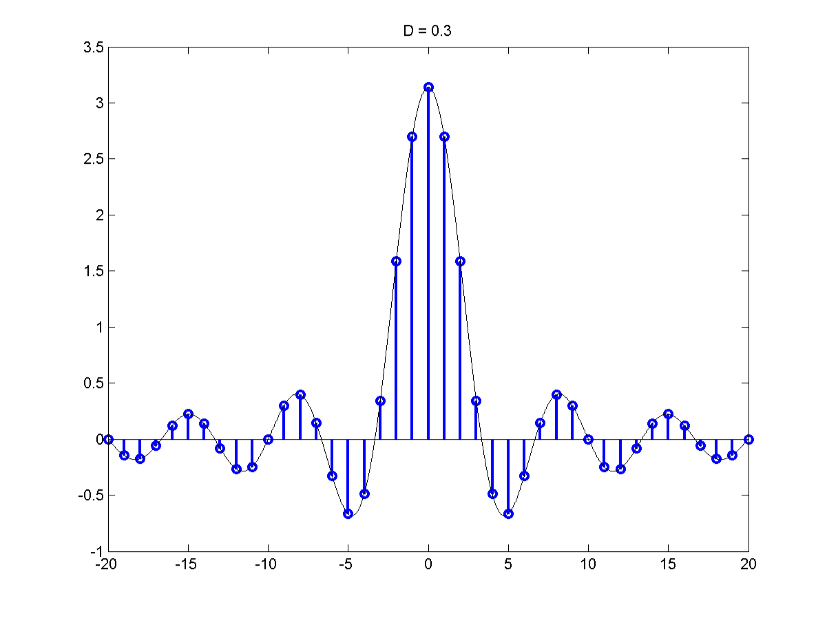
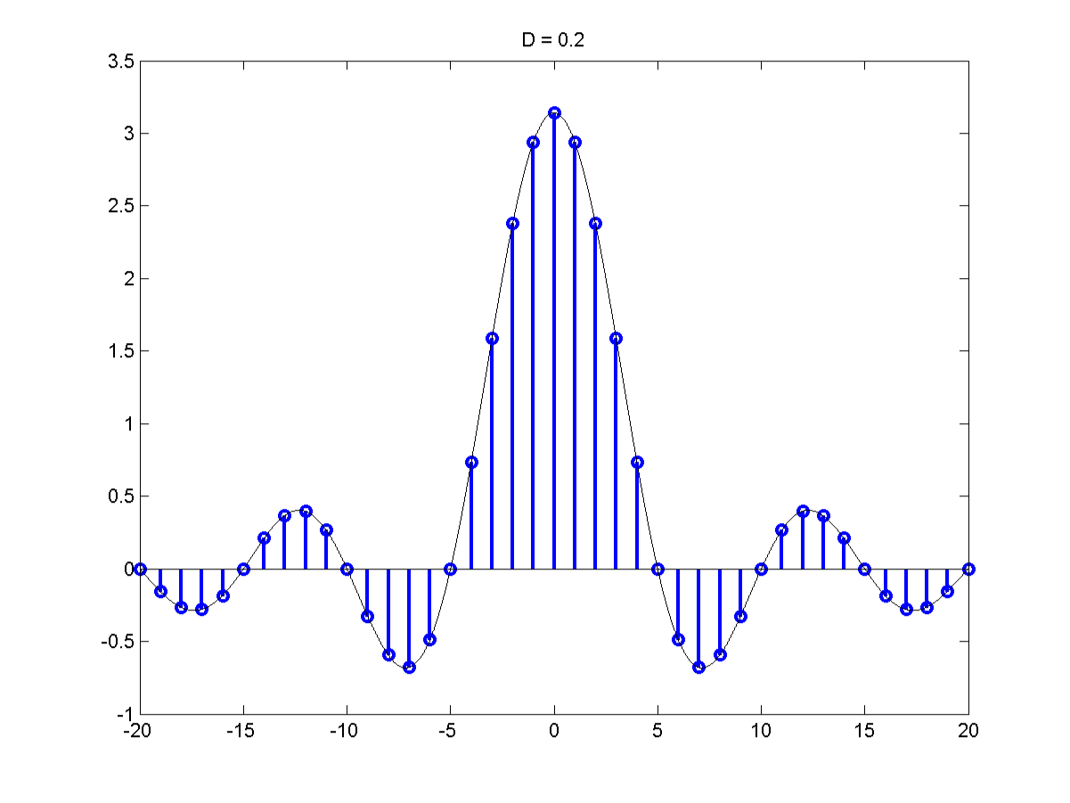
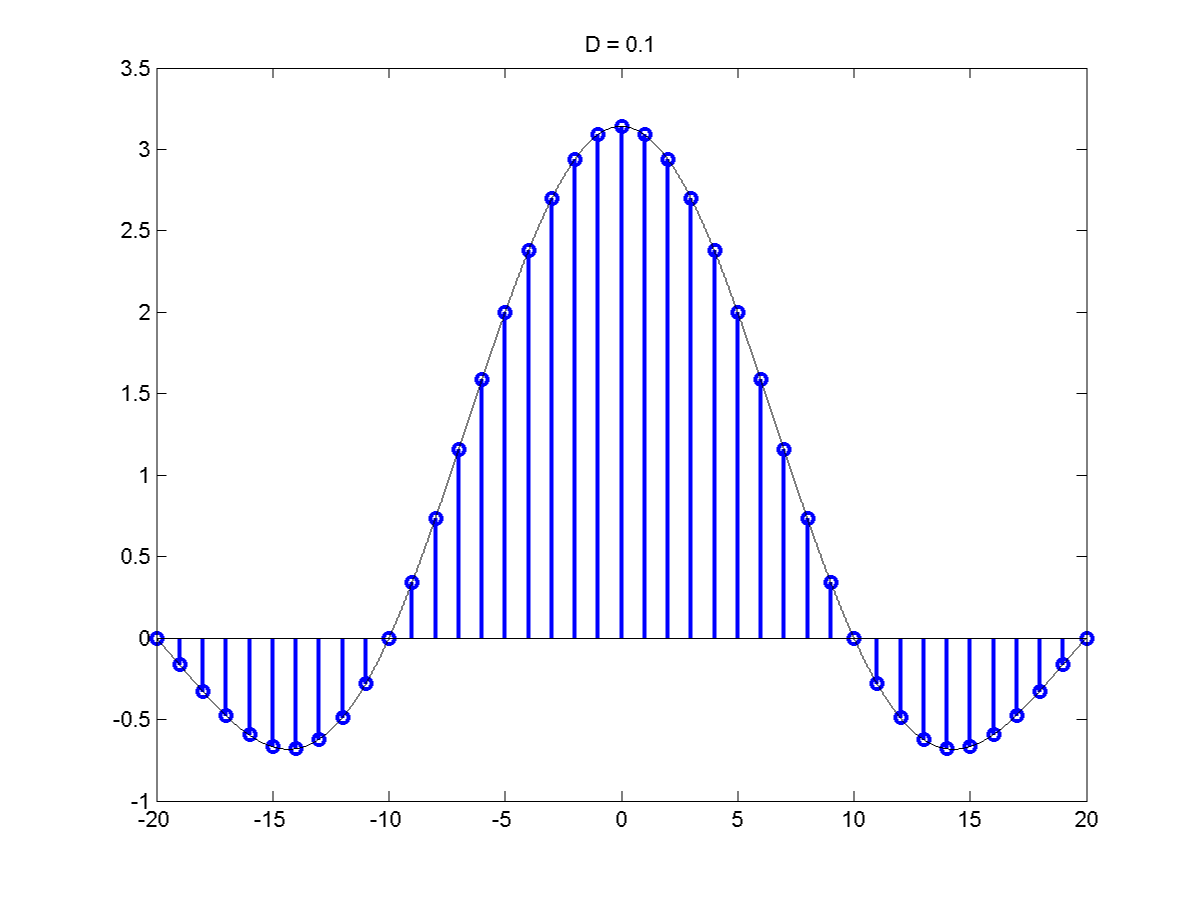
Now consider a modified pulse train where the height of the pulses is $\frac{1}{d}$ (so that the area of the pulse is 1).
\[C_k = \frac{D}{d}sinc \pi k D = \frac{1}{T} sinc \pi k D\]
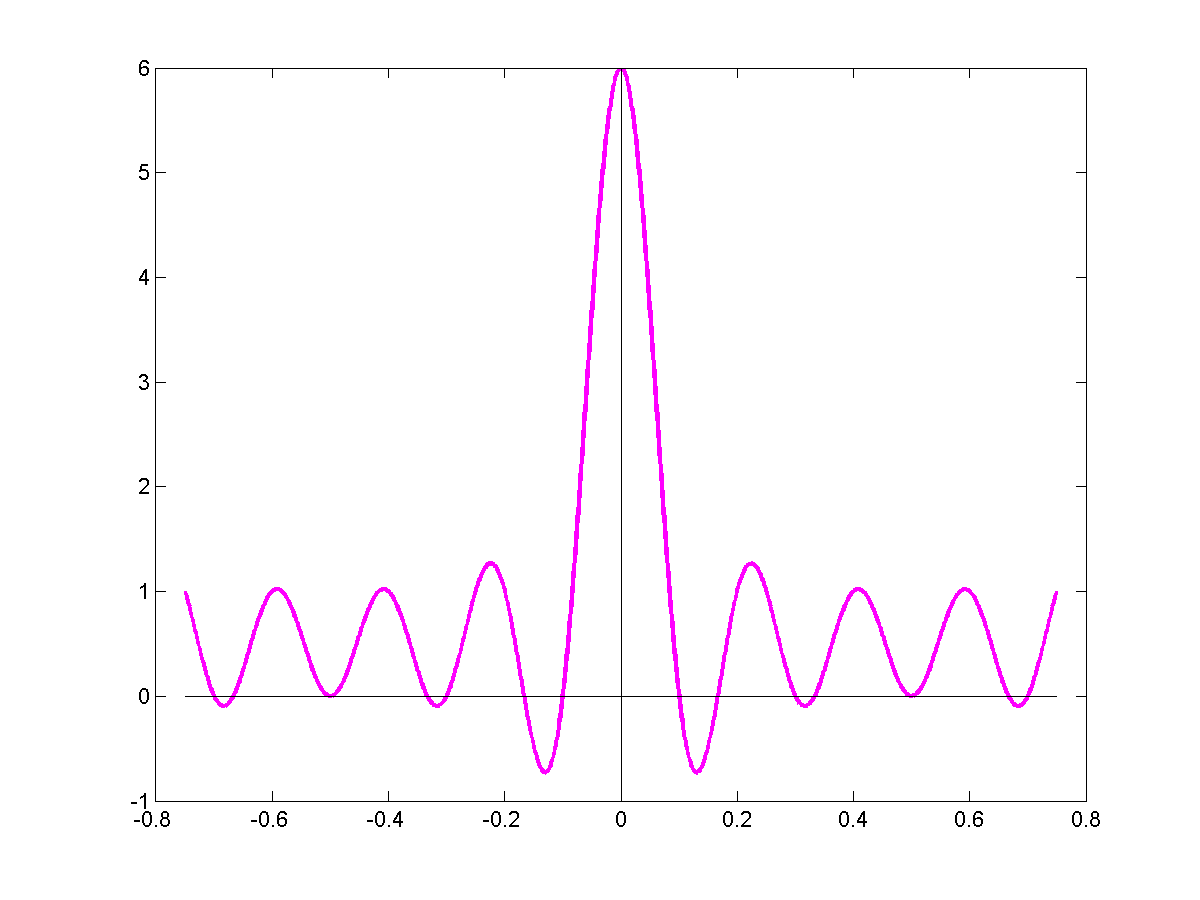
Recall the shape of a sinc function.
The sinc function goes to 0 at $\pm \pi$. Most of the area under the sinc lies between $- \pi$ & $\pi$ so must of the F.S. cooeficients will also lie
between $- \pi$ & $\pi$. The coefficient at $\pi$ is
\[\pi kD = \pi\]
\[\Rightarrow k = \frac{1}{D}\]
The total nuber of coefficients between the frequency at $k = \frac{1}{D}$ is $\frac{2 \pi}{TD}$
The bandwidth $\Delta w = \frac{4 \pi}{TD}$
\[\Delta wT = \frac{4 \pi}{D}]
Bandwidth x priod = $\frac{4 \pi}{D}$
This the uncertainty principle $\frac{4 \pi}{D}$ is the number of distinct frequencies.
As T decreases we can distinguish higher & higher frequencies for instance as out time resolution goes up. But if D is fixed as T decreases
$\delta w$ goes up and out ability to distinguish between nearby frequencies goes down.
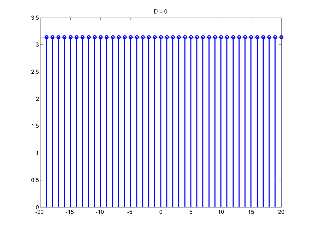
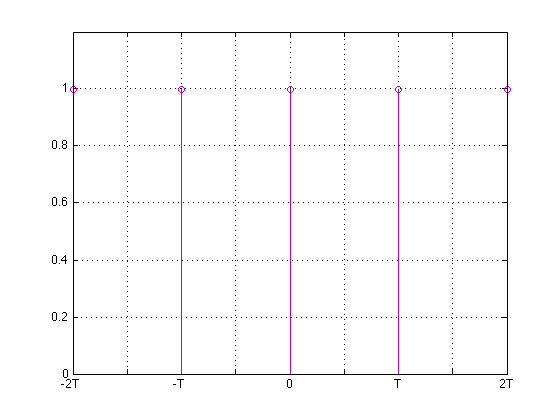
This is a key observation. At D = 0,
\[s(t) = \sum_{k=-\infty}^{\infty} \delta(t - k \tau)\]
For example a pulse train:
\[C_k = \frac{1}{T} \forall k\]
A pulse train in time becomes a pulse train the F.S. coefficients or a pulse train in frequency.
Back